I’m pleased to have recently had my first article published on the Oracle Technology Network (OTN). You can read it in its full splendour and glory(!) over there, but I thought I’d give a bit of background to it and the tools demonstrated within.
OBIEE Performance Analytics Dashboards
One of the things that we frequently help our clients with is reviewing and optimising the performance of their OBIEE systems. As part of this we’ve built up a wealth of experience in the kind of suboptimal design patterns that can cause performance issues, as well as how to go about identifying them empirically. Getting a full stack view on OBIEE performance behaviour is key to demonstrating where an issue lies, prior to being able to resolve it and proving it fixed, and for this we use the Rittman Mead OBIEE Performance Analytics Dashboards.
A common performance issue that we see is analyses and/or RPDs built in such a way that the BI Server inadvertently returns many gigabytes of data from the database and in doing so often has to dump out to disk whilst processing it. This can create large NQS_tmp files, impacting the disk space available (sometimes critically), and the disk I/O subsystem. This is the basis of the OTN article that I wrote, and you can read the full article on OTN to find out more about how this can be a problem and how to go about resolving it.
OBIEE implementations that cause heavy use of temporary files on disk by the BI Server can result in performance problems. Until recently in OBIEE, it was really difficult to track because of the transitory nature of the files. By the time the problem had been observed (for example, disk full messages), the query responsible had moved on and so the temporary files deleted. At Rittman Mead we have developed lightweight diagnostic tools that collect, amongst other things, the amount of temporary disk space used by each of the OBIEE components.
This can then be displayed as part of our Performance Analytics Dashboards, and analysed alongside other performance data on the system such as which queries were running, disk I/O rates, and more:
Because the Performance Analytics Dashboards are built in a modular fashion, it is easy to customise them to suit specific analysis requirements. In this next example you can see performance data from Oracle being analysed by OBIEE dashboard page in order to identify the cause of poorly-performing reports:
We’ve put online a set of videos here demonstrating the Performance Analytics Dashboards, and explaining in each case how they can help you quickly and accurately diagnose OBIEE performance problems.
Elastic announced their Graph tool at ElastiCON 2016 (see presentation here). It’s part of the forthcoming X-Pack which bundles Graph along with other helper tools such as Shield and Marvel. Graph itself is two things; an extension of Elasticsearch’s capabilities, enabling the user to explore how items indexed in Elasticsearch are related, and a plugin for Kibana that acts as an optional front-end for this new functionality.
You can find a good introduction to Graph and the purpose and theory behind it in the documentation here. The installation of the components themselves is simple and documented here.
First Graph
To use Graph, you just point it at your existing data in Elasticsearch. The first data set I’m going to explore is one of the standard ones that everyone uses; Twitter. I’m streaming it in through Logstash (via Kafka for flexibility), but if you wanted you could ship it in via JDBC from any RDBMS, or from HDFS too. See an important note at the end of this article about the slice of data within it, because it affects how the relationships visualised here should be viewed.
On launching Kibana’s Graph plugin (http://localhost:5601/app/graph) I choose the index (note that index patterns, e.g. when partitioning by date, are not supported yet), and the field in the data that I want to use as my vertices. A point to note here – “vertices” are usually called “nodes” in Graph terminology, but since Elasticsearch already uses “nodes” as part of its infrastructure topology terminology, they had to pick a different term.
In the search box, I can put my search term from which I’m interested to see the related ‘vertices’.
Sounds baffling? It is, kinda – right up until you run it (hit enter from the search box or click the magnifying glass search icon) and see what happens:
Here we’re seeing the hashtags used in tweets that mention Kibana. The “connections” (Elastic term) or “edges” (general Graph term) show which vertices (nodes) are related, and the width indicates the strength of that relationship (based on Elasticsearch’s significant terms and scoring algorithm). For more details, see the “Behind the Scenes” section towards the end of this article.
We can add in a second set of vertices by running a second search (“Elasticsearch”) – the results for these are, in effect, appended to the existing ones:
Add Links
Since we’ve pulled back an additional set of vertices, it could be that there’s overlap between these and the first set (you’d kinda of expect it, Elasticsearch and Kibana being related). To visualise this, use the Add Links button
Note how the graph redraws itself with additional connections:
Blinked and you missed it? Use the Undo button to step back, and Redo button to re-apply.
Grouping Vertices
If you look closely at the graph you’ll see that Elasticsearch, ElasticSearch, and elasticsearch are all there as separate vertices. This is because I’m using a non-analyzed index field, so the strings are treated literally, case included. In this specific example, we’d probably re-run the graph using the analysed version of the field, which following the same two searches as above gives this:
But, sticking with our non-analysed example, we can use it to demonstrate Graph’s ability to group multiple terms together into a single vertex. Switch to Advanced Mode:
and then select the three vertices and click the group option
Now all three, and their connections, are as one:
Whilst the above analysed/non-analysed difference gave me excuse to show the group function (can you tell I’ve done many-a-failed-live-demo? ;-) ), I’m now going to switch over to a graph built on the analysed version of the hashtag field, as we saw briefly above:
Tidying up the Graph – Delete and Blacklist
There’s a few straglers on the Graph that are making it less easy to comprehend. We can temporarily remove them, or even blacklist them from appearing again in this session:
Expand Selection
One of the points of Graph analysis is visualising the relationships in your data in a way that standard relational methods may not lend themselves to so easily. We can now start to explore this further, by digging into the Graph that we’ve got so far. This process, along with the add links seen above, is often called “spidering“. By selecting the elasticsearch node and clicking on Expand selection we can see additional (by default, five) vertices related to this one:
So we see that kafka is related to Elasticsearch (in the view of the twitterati, at least), and let’s expand that Kafka vertex too:
By clicking the Expand selection button again for the same vertex we get further results added:
We can select one node (e.g. realtime) an using the Add Link see additional relationships:
But, there are many nodes, and we want to see any relationships. So, switch to Advanced Mode, select All…
…add Add Link again:
Knob Twiddling
Let’s start with a blank canvas, in basic mode, showing hashtags related to … me (@rmoff)!
But, surely I do more than talk about OBIEE and ODI? Like, Elasticsearch? Let’s relax the Graph selection criteria, under Settings:
and run the search again (on top of the existing results):
There’s more results … but I know how much I tweet and it feels like I’m only seeing a part of the picture. By switching over to Advanced Mode, we can refine how many results each field returns:
I reset the workspace (undo to blank, or just reload), and run the search again, this time with a greater number of hashtag field values shown, and with the same relaxed search settings as shown above:
At this point I’m into “fiddling” territory, twiddling with the ‘Number of terms’, ‘Significant’ and ‘Certainty’ knobs to see how the results vary. You can read more about the algorithm behind the Significance setting here, and more about the Graph API here. The certainty setting is simply “The min number of documents that are required as evidence before introducing a related term”, so by lowering it we see more links, but potentially with more “noise” too, of terms that aren’t really related.
An important point to note here is the dataset that I’m using is already biased because of the terms I’m including in my twitter feed search, therefore I’d expect to see this skew in the results below. See the section at the end of this article for more details of the dataset.
Based on the above, “Significant” seems to reduce the number of relationships discovered, but increase the level of weight shown in those that are there.
Adding Additional Vertex Fields
So we’ve seen a basic overview of how to generate Graphs, expand selections, and add relationships to those additional selections. Let’s look now at how multiple fields can be added to a Graph.
Starting with a blank workspace, I switched to Advanced Mode and added two fields from my twitter data:
user.screen_name
in_reply_to_screen_name
Note that you can customise the colour and icon of different fields.
Under Options I’ve left Significant Links enabled, and set Certainty to 1.
Let’s see who’s been interacting about the recent E4 summit:
Whilst it looks like Mark Rittman is the centre of everything, this is actually highlighting a skew in the source dataset – which includes everything Mark tweets but not all tweets about E4. See the section at the end of this article for more details of the dataset.
The lower cluster is Mark as the addressee of tweets (i.e. he is the in_reply_to_screen_name), whilst the upper cluster is tweets that Mark has sent addressing others (i.e. he is the user.screen_name).
If we click on Add Links a couple of times we can see that there’s other connections here – for example, Mark replies to Stewart (@stewartbryson), who Christian Berg (@Nephentur) talks to, who in turn talks to Mark.
This being twitter and the age of narcissism, I’ll click on my vertex and click Expand Selection to see the people who in turn talk to me:
And by using Add Link see how they relate to those already shown in the Graph:
Viewing Associated Records
Within Graph there’s the option to view the data associated with one or more vertices. We do this by selecting a vertex and clicking on View Example Docs (in Elasticsearch parlance, a document is akin to a ‘row’ as traditional RDBMS folk would know it). From here select the field – for twitter the text field has the contents of the tweet:
Adding Even more Vertex Fields
So, we’ve got a bit of a picture of who talks to whom, but can we see what they’re talking about? We could use the text field shown above to see the contents of tweets but that’s down in the weeds of individual tweets – we want to step back a notch and get a summarised view.
First I add in the hashtag field:
And then deselect the two username fields. This is so that I can expand existing vertices, and instead of showing related hashtags and users, instead I only expand it to show hashtags – and not additional users.
Now I select Mark as the orinator of a tweet, and Expand Selection followed by Add Links on all vertices until I get this:
The number of values selected is key in getting a representative Graph. Above I used a value of 10. Compare that to instead running the same process but with 50. Under Options I’ve left Significant Links enabled, and set Certainty to 1:
One interesting point we can see from this is that the user “itknowingness” in the cluster on the left seems to use all the hashtags, but doesn’t interact with anyone – from the Graph it’s easy to see, and a great example of where Graph gives you the answer to a question you didn’t necessarily know that you had, and which to get the answer out through a traditional RDBMS query would need a very specific query to do so. Looking at the source data via Kibana’s Discover panel shows that it is indeed a bot auto-retweeting anything and everything:
Building a Graph from Scratch
Now that we’ve seen all the salient functions, let’s start with a blank canvas, and see where we get.
The setttings I’m using are:
Significant Links unticked
Certainty = 1
Field entities.hashtags.text.analyzed max terms = 10
Field user.screen_name max terms = 10
Initial search term rmoff
Then I click on markrittman and Expand Selection, the same for mrainey, and also for the two hashtags e4 and hadoop:
Within the clusters, let’s see what links exist. With no vertices select I click on Add Links (which seems to be the same as selecting all vertices and doing the same). With each click additional links are added, all related to the hadoop/bigdata area:
I’m interested now in the E4 region of the Graph, and the vertices related to Mark Rittman. Clicking on his vertex and clicking “Select Neighbours” does exactly that:
Now I’m more interested in digging into the terms (hashtags) that are related that people, so I deselect the user.screen_name field, and then Expand Selection and Add Links again.
Note the width of the connections – a strong relationship between Mark Rittman, “Hadoop” and “SQL”, which is presumably from the tweets around the presentation he did recently on the subject of… SQL on Hadoop. Other terms, including Hive and Impala, are also related, as you’d expect.
Graphing Tweet Text Contents
By making sure that the tweet text is available as an analysed field we can produce a Graph based on the ‘tokens’ within the tweet, rather than the literal 140 characters. Whilst hashtags are there deliberately to help with the classification and grouping of tweets (so that other people can follow conversations on the same subject) there are two reasons why you’d want to look at the tweet text too:
Not everyone uses hashtags
Not all relationships are as boolean as a hashtag or not – maybe a general discussion in an area re-uses the same words which overall forms a relationship between the terms.
Here I’m going back to the default settings:
Significant Links ticked
Certainty = 3
And returning two fields – hashtag and tweet text
Field entities.hashtags.text.analyzed max terms = 20
Field text.analyzed max terms = 50
Initial search term kafka
I then tidy it up a bit :
Joining the same/near-same text and hashtags, such as “kafkasummit” hashtag and the same text. If you think about the contents of a tweet, hashtags are part of the text, therefore, there’s going to be a lot of this duplication.
Blacklisted text terms that are URL snippets. Here I’m using the Example Docs function to check the context of the term in the whole text field
I also blacklisted common words (“the”, “of”, etc), and foreign ones (how British…).
Behind the Scenes
The Kibana Graph plugin is just a front-end for the Graph extension in Elasticsearch. It’s useful (and fun!) for exploring data, but in practice you’d be making direct REST API calls into Elasticsearch to retrieve a list of vertices and connections and relative weights for use in your application. You can see details of this from the Settings page and Last Request option
Looking at an example (the one used in the first example on this article), the request is pretty simple:
Note how the connections are described using the relative (zero-based) instance number of the vertices. You can also see that the width of a connection is based on the weight (calculated from the significant terms algorithm), rather than document count. Compare the connection width of timelion/kibana (vertices 1 and 5 respectively), with a weighting of 0.33 (kibana -> timelion) and 0.045 (timelion -> kibana) but overlapping document count of 29:
with elasticsearch -> kibana that has an overlapping document count of 80 but only a weight of 0.0001.
Elasticsearch’s documentation describes the significant terms algorithm thus, using the example of suggesting “H5N1” when users search for “bird flu” in text:
In all these cases the terms being selected are not simply the most popular terms in a set. They are the terms that have undergone a significant change in popularity measured between a foreground and background set. If the term “H5N1” only exists in 5 documents in a 10 million document index and yet is found in 4 of the 100 documents that make up a user’s search results that is significant and probably very relevant to their search. 5/10,000,000 vs 4/100 is a big swing in frequency.
So from this, we can roughly say that Graph is looking at the number of documents in which timelion is mentioned as a proportion of the whole dataset, and then in the number of documents in which the hashtag Kibana exists and also timelion is mentioned. Since the former is a plugin of the latter, the close relationship would be expected. You can use Kibana to explore the significant terms concept further – for example, taking the same ‘seed’ as the original Graph query above, Kibana, gives a similar set of results as the Graph:
More information about the scoring can be found here, which includes the fact that the scoring is, in part, based on TF-IDF (Term Frequency-Inverse Document Frequency).
This tool is a great way to dip one’s toe into the waters of Graph analysis and visualisation. It’s another approach to consider in the data discovery phase of your analytics work, when you don’t even know the questions that you’ve got for the data in front of you. Your data can remain in Elasticsearch in the same format it’s always been, and the Graph function just runs on top of it.
I’ll not profess to be a Graph theory expert, so can’t pass much comment on the theoretical rigour of the results and techniques seen. One thing that struck me with it was that there’s no (apparent) way to manually influence the weight of connections and vertices – for example, based on the number of followers someone has one twitter consider them more (or less) relevant when determining relationships.
The dataset I’m using is a live stream from Twitter, via Logstash and Kafka, searching for a set of terms related to me and the field I work in. Therefore, there’s going to be a bunch of relationships missing (if I’ve not included the relevant term in my tweet search), and relationships over-stated (because as a proportion of all the records the terms I’ve selected will dominate).
An interesting use of Graph (or Elasticsearch’s significant terms aggregation in general) could be to identify all the relevant terms that I should be including in my twitter search, by sampling an ‘unpolluted’ feed for relationships. For example, if I’m interested in capturing Kafka tweets, perhaps I should also be capturing those related to Samza, Spark, and so on.
OBIEE 12c has changed quite a lot in how it manages configuration. In OBIEE 11g configuration was based around system MBeans and the biee-domain.xml as the master copy of settings – and if you updated a configuration directly that was centrally managed, it would get reverted back. Now in OBIEE 12c configuration can be managed directly in text files again – but also through EM still (not to mention WLST). Confused? Yep, I was.
In the configuration files such as NQSConfig.INI there are settings still marked with the ominous comment:
# This Configuration setting is managed by Oracle Enterprise Manager Fusion Middleware Control
In 11g this meant – dragons be here; turn back all ye who don’t want to have your configuration settings wiped next time the stack boots.
Now in 12c, I can make a configuration change (such as enabling BI Server caching), restart the affected component, and the change will take affect — and persist through a restart of the whole OBIEE stack. All good.
But … the fly in the ointment. If I restart just the affected component (for example, BI Server for an NQSConfig.INI change), since I don’t want to waste time bouncing the whole stack if I don’t need to, then Enterprise Manager will continue to show the old setting:
So even though in fact the cache is enabled (and I can see entries being populated in it), Enterprise Manager suggests that it’s not. Confusing.
So … if we’re going to edit configuration files by hand (and personally I prefer to, since it saves firing up a web browser), we need to know how to make sure Enterprise Manager will to reflect the change too. Does EM poll the file whilst running? Or something direct to each component to request the configuration? Or maybe it just reads the file on startup only?
Enter sysdig! What I’m about to use it for is pretty darn trivial (and could probably be done with other standard *nix tools), but is still a useful example. What we want to know is which process reads NQSConfig.INI, and from there isolate the particular component that we need to restart to get it to trigger a re-read of the file and thus correctly show the value in Enterprise Manager.
I ran sysdig with a filter for filename and custom output format to include the process PID:
sudo sysdig -A -p "%evt.num %evt.time %evt.cpu %proc.name (%proc.pid) %evt.dir %evt.info" "fd.filename=NQSConfig.INI and evt.type=open"
Nothing was written (i.e. nothing was polling the file), until I bounced the full OBIEE stack ($DOMAIN_HOME/bitools/bin/stop.sh && $DOMAIN_HOME/bitools/bin/start.sh). During the startup of the AdminServer, sysdig showed:
It’s AdminServer — which makes sense, because Enterprise Manager is a java deployment hosted in AdminServer.
So, if you want to hack the config files by hand, restart either the whole OBIEE stack, or the affected component plus AdminServer in order for Enterprise Manager to pick up the change.
The OBIEE BI Server cache can be a great way of providing a performance boost to response times for end users – so long as it’s implemented carefully. Done wrong, and you’re papering over the cracks and heading for doom; done right, and it’s the ‘icing on the cake’. You can read more about how to use it properly here, and watch a video I did about it here. In this article we’ll see how the BI Server cache has changed in OBIEE 12c in a way that could prove somewhat perplexing to developers used to OBIEE 11g.
The BI Server cache works by inspecting queries as they are sent to the BI Server, and deciding if an existing cache entry can be used to provide the data. This can include direct hits (i.e. the same query being run again), or more advanced cases, where a subset or aggregation of an existing cache entry could be used. If a cache entry is used then a trip to the database is avoided and response times will typically be better – particularly if more than one database query would have been involved, or lots of additional post-processing on the BI Server.
When an analysis or dashboard is run, Presentation Services generates the necessary Logical SQL to return the data needed, and sends this to the BI Server. It’s at this point that the cache will, or won’t, kick in. The BI Server will accept Logical SQL from other sources than Presentation Services – in fact, any JDBC or ODBC client. This is useful as it enables us to validate behaviour that we’re observing and see how it can apply elsewhere.
When you build an Analysis in OBIEE 11g (and before), the cache will be used if applicable. Each time you add a column, or hit refresh, you’ll get an entry back from the cache if one exists. This has benefits – speed – but disadvantages too. When the data in the database changes, you will still get a cache hit, regardless. The only way to force OBIEE to show you the latest version of the data is to purge the cache first. You can target cache purges based on databases, tables, or even specific queries – but you do need to purge it.
What’s changed in OBIEE 12c is that when you click “Refresh” on an Analysis or Dashboard, the query is re-run against the source and the cache re-populated. Even if you have an existing cache entry, and even if the underlying data has not changed, if you hit Refresh, the cache will not be used. Which kind of makes sense, since “refresh” probably should indeed mean that.
Digging into OBIEE Cache Behaviour
Let’s prove this out. I’ve got SampleApp v506 (OBIEE 11.1.1.9), and SampleApp v511 (OBIEE 12.2.1). First off, I’ll clear the cache on each, using call saPurgeAllCache();, run via Issue SQL:
Then I can use another BI Server procedure call to view the current cache contents (new in 11.1.1.9), call NQS_GetAllCacheEntries(). For this one particularly make sure you’ve un-ticked “Use Oracle BI Presentation Services Cache”. This is different from the BI Server cache which is the subject of this article, and as the name implies is a cache that Presentation Services keeps.
I’ve confirmed that the BI Server cache is enabled on both servers, in NQSConfig.INI
###############################################################################
#
#  Query Result Cache Section
#
###############################################################################


[CACHE]

ENABLE = YES;  # This Configuration setting is managed by Oracle Enterprise Manager Fusion Middleware Control
Now I create a very simple analysis in both 11g and 12c, showing a list of Airline Carriers and their Codes:
After clicking Results, a cache entry is inserted on each respective system:
Of particular interest is the create time, last used time, and number of times used:
If I now click Refresh in the Analysis window:
We see this happen to the caches:
In OBIEE 11g the cache entry is used – but in OBIEE 12c it’s not. The CreatedTime is evidently not populated correctly, so instead let’s dive over to the query log (nqquery/obis1-query in 11g/12c respectively). In OBIEE 11g we’ve got:
-- SQL Request, logical request hash:
7c365697
SET VARIABLE QUERY_SRC_CD='Report',PREFERRED_CURRENCY='USD';SELECT
   0 s_0,
   "X - Airlines Delay"."Carrier"."Carrier Code" s_1,
   "X - Airlines Delay"."Carrier"."Carrier" s_2
FROM "X - Airlines Delay"
ORDER BY 1, 3 ASC NULLS LAST, 2 ASC NULLS LAST
FETCH FIRST 5000001 ROWS ONLY

-- Cache Hit on query: [[
Matching Query: SET VARIABLE QUERY_SRC_CD='Report',PREFERRED_CURRENCY='USD';SELECT
   0 s_0,
   "X - Airlines Delay"."Carrier"."Carrier Code" s_1,
   "X - Airlines Delay"."Carrier"."Carrier" s_2
FROM "X - Airlines Delay"
ORDER BY 1, 3 ASC NULLS LAST, 2 ASC NULLS LAST
FETCH FIRST 5000001 ROWS ONLY
Whereas 12c is:
-- SQL Request, logical request hash:
d53f813c
SET VARIABLE OBIS_REFRESH_CACHE=1,QUERY_SRC_CD='Report',PREFERRED_CURRENCY='USD';SELECT
   0 s_0,
   "X - Airlines Delay"."Carrier"."Carrier Code" s_1,
   "X - Airlines Delay"."Carrier"."Carrier" s_2
FROM "X - Airlines Delay"
ORDER BY 3 ASC NULLS LAST, 2 ASC NULLS LAST
FETCH FIRST 5000001 ROWS ONLY

-- Sending query to database named X0 - Airlines Demo Dbs (ORCL) (id: <<320369>>), connection pool named Aggr Connection, logical request hash d53f813c, physical request hash a46c069c: [[
WITH
SAWITH0 AS (select T243.CODE as c1,
     T243.DESCRIPTION as c2
from
     BI_AIRLINES.UNIQUE_CARRIERS T243 /* 30 UNIQUE_CARRIERS */ )
select D1.c1 as c1, D1.c2 as c2, D1.c3 as c3 from ( select 0 as c1,
     D1.c1 as c2,
     D1.c2 as c3
from
     SAWITH0 D1
order by c3, c2 ) D1 where rownum <= 5000001

-- Query Result Cache: [59124] The query for user 'prodney' was inserted into the query result cache. The filename is '/app/oracle/biee/user_projects/domains/bi/servers/obis1/cache/NQS__736117_52416_27.TBL'.
Looking closely at the 12c output shows three things:
OBIEE has run a database query for this request, and not hit the cache
A cache entry has clearly been created again as a result of this query
The Logical SQL has a request variable set: OBIS_REFRESH_CACHE=1
This is evidently added it by Presentation Services at runtime, since the Advanced tab of the analysis shows no such variable being set:
Let’s save the analysis, and experiment further. Evidently, the cache is being deliberately bypassed when the Refresh button is clicked when building an analysis – but what about when it is opened from the Catalog? We should see a cache hit here too:
Nope, no hit.
But, in the BI Server query log, no entry either – and the same on 11g. The reason being …. Presentation Service’s cache. D’oh!
From Administration > Manage Sessions I select Close All Cursors which forces a purge of the Presentation Services cache. When I reopen the analysis from the Catalog view, now I get a cache hit, in both 11g and 12c:
The same happens (successful cache hit) for the analysis used in a Dashboard being opened, having purged the Presentation Services cache first.
So at this point, we can say that OBIEE 11g and 12c both behave the same with the cache when opening analyses/dashboards, but differ when refreshing the analysis. In OBIEE 12c when an analysis is refreshed the cache is deliberately bypassed. Let’s check on refreshing a dashboard:
Same behaviour as with analyses – in 11g the cache is hit, in 12c the cache is bypassed and repopulated
To round this off, let’s doublecheck the behaviour of the new request variable that we’ve found, OBIS_REFRESH_CACHE. Since it appears that Presentation Services is adding it in at runtime, let’s step over to a more basic way of interfacing with the BI Server – nqcmd. Whilst we could probably use Issue SQL (as we did above for querying the cache) I want to avoid any more behind-the-scenes funny business from Presentation Services.
SET VARIABLE OBIS_REFRESH_CACHE=1,QUERY_SRC_CD='Report',PREFERRED_CURRENCY='USD';SELECT 0 s_0, "X - Airlines Delay"."Carrier"."Carrier Code" s_1, "X - Airlines Delay"."Carrier"."Carrier" s_2 FROM "X - Airlines Delay" ORDER BY 3 ASC NULLS LAST, 2 ASC NULLS LAST FETCH FIRST 5000001 ROWS ONLY
In `obis1-query.log’ there’s the cache bypass and populate:
Query Result Cache: [59124] The query for user 'prodney' was inserted into the query result cache. The filename is '/app/oracle/biee/user_projects/domains/bi/servers/obis1/cache/NQS__736117_53779_29.TBL'.
If I run it again without the OBIS_REFRESH_CACHE variable:
SET VARIABLE QUERY_SRC_CD='Report',PREFERRED_CURRENCY='USD';SELECT 0 s_0, "X - Airlines Delay"."Carrier"."Carrier Code" s_1, "X - Airlines Delay"."Carrier"."Carrier" s_2 FROM "X - Airlines Delay" ORDER BY 3 ASC NULLS LAST, 2 ASC NULLS LAST FETCH FIRST 5000001 ROWS ONLY
We get the cache hit as expected:
-------------------- Cache Hit on query: [[
Matching Query: SET VARIABLE OBIS_REFRESH_CACHE=1,QUERY_SRC_CD='Report',PREFERRED_CURRENCY='USD';SELECT    0 s_0,    "X - Airlines Delay"."Carrier"."Carrier Code" s_1,    "X - Airlines Delay"."Carrier"."Carrier" s_2 FROM "X - Airlines Delay" ORDER BY 3 ASC NULLS LAST, 2 ASC NULLS LAST FETCH FIRST 5000001 ROWS ONLY
Created by:     prodney
Out of interest I ran the same two tests on 11g — both resulted in a cache hit, since it presumably ignores the unrecognised variable.
Summary
In OBIEE 12c, if you click “Refresh” on an analysis or dashboard, OBIEE Presentation Services forces a cache-bypass and cache-reseed, ensuring that you really do see the latest version of the data from source. It does this using the request variable, new in OBIEE 12c, OBIS_REFRESH_CACHE.
One of the big changes in OBIEE 12c for end users is the ability to upload their own data sets and start analysing them directly, without needing to go through the traditional data provisioning and modelling process and associated leadtimes. The implementation of this is one of the big architectural changes of OBIEE 12c, introducing the concept of the Extended Subject Areas (XSA), and the Data Set Service (DSS).
In this article we’ll see some of how XSA and DSS work behind the scenes, providing an important insight for troubleshooting and performance analysis of this functionality.
What is an XSA?
An Extended Subject Area (XSA) is made up of a dataset, and associated XML data model. It can be used standalone, or “mashed up” in conjunction with a “traditional” subject area on a common field
How is an XSA Created?
At the moment the following methods are available:
“Add XSA” in Visual Analzyer, to upload an Excel (XLSX) document
CREATE DATASET logical SQL statement, that can be run through any interface to the BI Server, including ‘Issue Raw SQL’, nqcmd, JDBC calls, and so on
Add Data Source in Answers. Whilst this option shouldn’t actually be present according to a this doc, it will be for any users of 12.2.1 who have uploaded the SampleAppLite BAR file so I’m including it here for completeness.
Under the covers, these all use the same REST API calls directly into datasetsvc. Note that these are entirely undocumented, and only for internal OBIEE component use. They are not intended nor supported for direct use.
How does an XSA work?
External Subject Areas (XSA) are managed by the Data Set Service (DSS). This is a java deployment (datasetsvc) running in the Managed Server (bi_server1), providing a RESTful API for the other OBIEE components that use it.
The end-user of the data, whether it’s Visual Analyzer or the BI Server, send REST web service calls to DSS, storing and querying datasets within it.
Where is the XSA Stored?
By default, the data for XSA is stored on disk in SINGLETON_DATA_DIRECTORY/components/DSS/storage/ssi, e.g. /app/oracle/biee/user_projects/domains/bi/bidata/components/DSS/storage/ssi
There’s a set of DSS-related tables installed in the RCU schema BIPLATFORM, which hold information including the XML data model for the XSA, along with metadata such as the user that uploaded the file, when they uploaded, and then name of the file on disk:
How Can the Data Set Service be Configured?
The configuration file, with plenty of inline comments, is at ORACLE_HOME/bi/endpointmanager/jeemap/dss/DSS_REST_SERVICE.properties. From here you con update settings for the data set service including upload limits as detailed here.
XSA Performance
Since XSA are based on flat files stored in disk, we need to be very careful in their use. Whilst a database may hold billions of rows in a table with with appropriate indexing and partitioning be able to provide sub-second responses, a flat file can quickly become a serious performance bottleneck. Bear in mind that a flat file is just a bunch of data plopped on disk – there is no concept of indices, blocks, partitions — all the good stuff that makes databases able to do responsive ad-hoc querying on selections of data.
If you’ve got a 100MB Excel file with thousands of cells, and want to report on just a few of them, you might find it laggy – because whether you want to report on them on or not, at some point OBIEE is going to have to read all of them regardless. We can see how OBIEE is handling XSA under the covers by examining the query log. This used to be called nqquery.log in OBIEE 11g (and before), and in OBIEE 12c has been renamed obis1-query.log.
In this example here I’m using an Excel worksheet with 140,000 rows and 78 columns. Total filesize of the source XLSX on disk is ~55Mb.
First up, I’ll build a query in Answers with a couple of the columns:
The logical query uses the new XSA syntax:
SELECT
   0 s_0,
   XSA('prodney'.'MOCK_DATA_bigger_55Mb')."Columns"."first_name" s_1,
   XSA('prodney'.'MOCK_DATA_bigger_55Mb')."Columns"."foo" s_2
FROM XSA('prodney'.'MOCK_DATA_bigger_55Mb')
ORDER BY 2 ASC NULLS LAST
FETCH FIRST 5000001 ROWS ONLY
The query log shows
Rows 144000, bytes 13824000 retrieved from database query
Rows returned to Client 200
So of the 55MB of data, we’re pulling all the rows (144,000) back to the BI Server for it to then perform the aggregation on it, resulting in the 200 rows returned to the client (Presentation Services). Note though that the byte count is lower (13Mb) than the total size of the file (55Mb).
As well as aggregation, filtering on XSA data also gets done by the BI Server. Consider this example here, where we add a predicate:
In the query log we can see that all the data has to come back from DSS to the BI Server, in order for it to filter it:
Rows 144000, bytes 23040000 retrieved from database
Physical query response time 24.195 (seconds),
Rows returned to Client 0
Note the time taken by DSS — nearly 25 seconds. Compare this later on to when we see the XSA data served from a database, via the XSA Cache.
In terms of BI Server (not XSA) caching, the query log shows that a cache entry was written for the above request:
Query Result Cache: [59124] The query for user 'prodney' was inserted into the query result cache. The filename is '/app/oracle/biee/user_projects/domains/bi/servers/obis1/cache/NQS__736113_56359_0.TBL'
If I refresh the query in Answers, the data is fetched anew (per this changed behaviour in OBIEE 12c), and the cache repopulated. If I clear the Presentation Services cache and re-open the analysis, I get the results from the BI Server cache, and it doesn’t have to refetch the data from the Data Set Service.
Since the cache has two columns in, an attribute and a measure, I wondered if running a query with just the fact rolled up might hit the cache (since it has all the data there that it needs)
Unfortunately it didn’t, and to return a single row of data required BI Server to fetch all the rows again – although looking at the byte count it appears it does prune the columns required since it’s now just over 2Mb of data returned this time:
Rows 144000, bytes 2304000 retrieved from database
Rows returned to Client 1
Interestingly if I build an analysis with several more of the columns from the file (in this example, ten of a total of 78), the data returned from the DSS to BI Server (167Mb) is greater than that of the original file (55Mb).
Rows 144000, bytes 175104000
Rows returned to Client 1000
And this data coming back from the DSS to the BI Server has to go somewhere – and if it’s big enough it’ll overflow to disk, as we can see when I run the above:
You can read more about BI Server’s use of temporary files and the impact that it can have on system performance and particularly I/O bandwidth in this OTN article here.
So – as the expression goes – “buyer beware”. XSA is an excellent feature, but used in its default configuration with files stored on disk it has the potential to wreak havoc if abused.
In a proper implementation you would follow in full the document, including provisioning a dedicated schema and tablespace for holding the data (to make it easier to manage and segregate from other data), but here I’m just going to use the existing RCU schema (BIPLATFORM), along with the Physical mapping already in the RPD (10 - System DB (ORCL)):
In NQSConfig.INI, under the XSA_CACHE section, I set:
ENABLE = YES;

# The schema and connection pool where the XSA data will be cached.
PHYSICAL_SCHEMA = "10 - System DB (ORCL)"."Catalog"."dbo";
CONNECTION_POOL = "10 - System DB (ORCL)"."UT Connection Pool";
Per the document, note that in the BI Server log there’s an entry indicating that the cache has been successfully started:
[101001] External Subject Area cache is started successfully using configuration from the repository with the logical name ssi.
[101017] External Subject Area cache has been initialized. Total number of entries: 0 Used space: 0 bytes Maximum space: 107374182400 bytes Remaining space: 107374182400 bytes. Cache table name prefix is XC2875559987.
Now when I re-run the test XSA analysis from above, returning three columns, the BI Server goes off and populates the XSA cache table:
-- Sending query to database named 10 - System DB (ORCL) (id: <<79879>> XSACache Create table Gateway), connection pool named UT Connection Pool, logical request hash b4de812e, physical request hash 5847f2ef:
CREATE TABLE dbo.XC2875559987_ZPRODNE1926129021 ( id3209243024 DOUBLE PRECISION, first_n[..]
Or rather, it doesn’t, because PHYSICAL_SCHEMA seems to want the literal physical schema, rather than the logical physical one (?!) that the USAGE_TRACKING configuration stanza is happy with in referencing the table.
Properties: description=<<79879>> XSACache Create table Exchange; producerID=0x1561aff8; requestID=0xfffe0034; sessionID=0xfffe0000; userName=prodney;
[nQSError: 17001] Oracle Error code: 1918, message: ORA-01918: user 'DBO' does not exist
I’m trying to piggyback on SA511’s existing configruation, which uses catalog.schema notation:
Instead of the more conventional approach to have the actual physical schema (often used in conjunction with ‘Require fully qualified table names’ in the connection pool):
So now I’ll do it properly, and create a database and schema for the XSA cache – I’m still going to use the BIPLATFORM schema though…
Updated NQSConfig.INI:
[ XSA_CACHE ]

ENABLE = YES;

# The schema and connection pool where the XSA data will be cached.
PHYSICAL_SCHEMA = "XSA Cache"."BIEE_BIPLATFORM";
CONNECTION_POOL = "XSA Cache"."XSA CP";
After refreshing the analysis again, there’s a successful creation of the XSA cache table:
-- Sending query to database named XSA Cache (id: <<65685>> XSACache Create table Gateway), connection pool named XSA CP, logical request hash 9a548c60, physical request hash ccc0a410: [[
CREATE TABLE BIEE_BIPLATFORM.XC2875559987_ZPRODNE1645894381 ( id3209243024 DOUBLE PRECISION, first_name2360035083 VARCHAR2(17 CHAR), [...]
-- Sending query to database named XSA Cache (id: <<65685>> XSACache Collect statistics Gateway), connection pool named XSA CP, logical request hash 9a548c60, physical request hash d73151bb:
BEGIN DBMS_STATS.GATHER_TABLE_STATS(ownname => 'BIEE_BIPLATFORM', tabname => 'XC2875559987_ZPRODNE1645894381' , estimate_percent => 5 , method_opt => 'FOR ALL COLUMNS SIZE AUTO' ); END;
Although I do note that it is used a fixed estimate_percent instead of the recommendedAUTO_SAMPLE_SIZE. The table itself is created with a fixed prefix (as specified in the obis1-diagnostic.log at initialisation), and holds a full copy of the XSA (not just the columns in the query that triggered the cache creation):
With the dataset cached, the query is then run and the query log shows a XSA cache hit
External Subject Area cache hit for 'prodney'.'MOCK_DATA_bigger_55Mb'/Columns :
Cache entry shared_cache_key = 'prodney'.'MOCK_DATA_bigger_55Mb',
table name = BIEE_BIPLATFORM.XC2875559987_ZPRODNE2128899357,
row count = 144000,
entry size = 201326592 bytes,
creation time = 2016-06-01 20:14:26.829,
creation elapsed time = 49779 ms,
descriptor ID = /app/oracle/biee/user_projects/domains/bi/servers/obis1/xsacache/NQSXSA_BIEE_BIPLATFORM.XC2875559987_ZPRODNE2128899357_2.CACHE
with the resulting physical query fired at the XSA cache table (replacing what would have gone against the DSS web service):
-- Sending query to database named XSA Cache (id: <<65357>>), connection pool named XSA CP, logical request hash 9a548c60, physical request hash d3ed281d: [[
WITH
SAWITH0 AS (select T1000001.first_name2360035083 as c1,
     T1000001.last_name3826278858 as c2,
     sum(T1000001.foo2363149668) as c3
from
     BIEE_BIPLATFORM.XC2875559987_ZPRODNE1645894381 T1000001
group by T1000001.first_name2360035083, T1000001.last_name3826278858)
select D1.c1 as c1, D1.c2 as c2, D1.c3 as c3, D1.c4 as c4 from ( select 0 as c1,
     D102.c1 as c2,
     D102.c2 as c3,
     D102.c3 as c4
from
     SAWITH0 D102
order by c2, c3 ) D1 where rownum <= 5000001
It’s important to point out the difference of what’s happening here: the aggregation has been pushed down to the database, meaning that the BI Server doesn’t have to. In performance terms, this is a Very Good Thing usually.
Rows 988, bytes 165984 retrieved from database query
Rows returned to Client 988
Whilst it doesn’t seem to be recorded in the query log from what I can see, the data returned from the XSA Cache also gets inserted into the BI Server cache, and if you open an XSA-based analysis that’s not in the presentation services cache (a third cache to factor in!) you will get a cache hit on the BI Server cache. As discussed earlier in this article though, if an analysis is built against an XSA for which a BI Server cache entry exists that with manipulation could service it (eg pruning columns or rolling up), it doesn’t appear to take advantage of it – but since it’s hitting the XSA cache this time, it’s less of a concern.
If you change the underlying data in the XSA
The BI Server does pick this up and repopulates the XSA Cache.
The XSA cache entry itself is 192Mb in size – generated from a 55Mb upload file. The difference will be down to data types and storage methods etc. However, that it is larger in the XSA Cache (database) than held natively (flat file) doesn’t really matter, particularly if the data is being aggregated and/or filtered, since the performance benefit of pushing this work to the database will outweigh the overhead of storage space. Consider this example here, where I run an analysis pulling back 44 columns (of the 78 in the spreadsheet) and hit the XSA cache, it runs in just over a second, and transfers from the database a total of 5.3Mb (the data is repeated, so rolls up):
Rows 1000, bytes 5576000 retrieved from database
Rows returned to Client 1000
If I disable the XSA cache and run the same query, we see this:
Rows 144000, bytes 801792000 Retrieved from database
Physical query response time 22.086 (seconds)
Rows returned to Client 1000
That’s 764Mb being sent back for the BI Server to process, which it does by dumping a whole load to disk in temporary work files:
As a reminder – this isn’t “Bad”, it’s just not optimal (response time of 50 seconds vs 1 second), and if you scale that kind of behaviour by many users with many datasets, things could definitely get hairy for all users of the system. Hence – use the XSA Cache.
As a final point, with the XSA Cache being in the database the standard range of performance optimisations are open to us – indexing being the obvious one. No indexes are built against the XSA Cache table by default, which is fair enough since OBIEE has no idea what the key columns on the data are, and the point of mashups is less to model and optimise the data but to just get it up there in front of the user. So you could index the table if you knew the key columns that were going to be filtered against, or you could even put it into memory (assuming you’ve licensed the option).
The MoS document referenced above also includes further performance recommendations for XSA, including the use of RAM Disk for XSA cache metadata files, as well as the managed server temp folder
Summary
External Subject Areas are great functionality, but be aware of the performance implications of not being able to push down common operations such as filtering and aggregation. Set up XSA Caching if you are going to be using XSA properly.
If you’re interested in the direction of XSA and the associated Data Set Service, this slide deck from Oracle’s Socs Cappas provides some interesting reading. Uploading Excel files into OBIEE looks like just the beginning of what the Data Set Service is going to enable!
New in Big Data Discovery 1.2 is the addition of BDD Shell, an integration point with Python. This exposes the datasets and BDD functionality in a Python and PySpark environment, opening up huge possibilities for advanced data science work on BDD datasets, particularly when used in conjunction with Jupyter Notebooks. With the ability to push back to Hive and thus BDD data modified in this environment, this is important functionality that will make BDD even more useful for navigating and exploring big data.
The Big Data Lite virtual machine is produced by Oracle for demo and development purposes, and hosts all the components that you’d find on the Big Data Appliance, all configured and integrated for use. Version 4.5 was released recently, which included BDD 1.2. In this article we’ll see how to configure BDD Shell on Big Data Lite 4.5 (along with Jupyter Notebooks), and in a subsequent post dive into how to actually use them.
Setting up BDD Shell on Big Data Lite
You can find the BDD Shell installation document here.
Login to BigDataLite 4.5 (oracle/welcome1) and open a Terminal window. The first step is to download Anaconda, which is a distribution of Python that also includes “[…] over 100 of the most popular Python, R and Scala packages for data science” as well as Jupyter notebook, which we’ll see in a moment.
cd ~/Downloads/
wget http://repo.continuum.io/archive/Anaconda2-4.0.0-Linux-x86_64.sh
Then install it: (n.b. bash is part of the command to enter)
bash Anaconda2-4.0.0-Linux-x86_64.sh
Accept the licence when prompted, and then select a install location – I used /u01/anaconda2 where the rest of the BigDataLite installs are
Anaconda2 will now be installed into this location:
/home/oracle/anaconda2

  - Press ENTER to confirm the location
  - Press CTRL-C to abort the installation
  - Or specify a different location below

[/home/oracle/anaconda2] >>> /u01/anaconda2
After a few minutes of installation, you’ll be prompted to whether you want to prepend Anaconda’s location to the PATH environment variable. I opted not to (which is the default) since Python is used elsewhere on the system and by prepending it it’ll take priority and possibly break things.
Do you wish the installer to prepend the Anaconda2 install location
to PATH in your /home/oracle/.bashrc ? [yes|no]
[no] >>> no
Now edit the BDD Shell configuration file (/u01/bdd/v1.2.0/BDD-1.2.0.31.813/bdd-shell/bdd-shell.conf) in your favourite text editor to add/amend the following lines:
Whilst BDD Shell is command-line based, there’s also the option to run Jupyter Notebooks (previous iPython Notebooks) which is a web-based interactive “Notebook”. This lets you build up scripts exploring and manipulating the data within BDD, using both Python and Spark. The big advantage of this over the command-line interface is that a ‘Notebook’ enables you to modify and re-run commands, and then once correct, retain them as a fully functioning script for future use.
To launch it, run:
cd /u01/bdd/v1.2.0/BDD-1.2.0.31.813/bdd-shell
/u01/anaconda2/bin/jupyter-notebook --port 18888
Important points to note:
It’s important that you run this from the bdd-shell folder, otherwise the BDD shell won’t initialise properly
By default Jupyter uses 8888, which is already in use on BigDataLite by Hue, so use a different one by specifying --port
Jupyter by default only listens locally, so you need to either be using BigDataLite desktop to run Firefox, or use port-forwarding if you want to access Jupyter from your local web browser.
Go to http://localhost:18888 in your web browser, and you should see the default Jupyter screen with a list of files:
In the next article, we’ll see how to use Jupyter Notebooks with Big Data Discovery, and get an idea of just how powerful the combination can be.
New in Big Data Discovery 1.2 is the addition of BDD Shell, an integration point with Python. This exposes the datasets and BDD functionality in a Python and PySpark environment, opening up huge possibilities for advanced data science work on BDD datasets. With the ability to push back to Hive and thus BDD data modified in this environment, this is important functionality that will make BDD even more useful for navigating and exploring big data.
Whilst BDD Shell is command-line based, there’s also the option to run Jupyter Notebooks (previous iPython Notebooks) which is a web-based interactive “Notebook”. This lets you build up scripts exploring and manipulating the data within BDD, using both Python and Spark. The big advantage of this over the command-line interface is that a ‘Notebook’ enables you to modify and re-run commands, and then once correct retain them as a fully functioning script for future use.
The Big Data Lite virtual machine is produced by Oracle for demo and development purposes, and hosts all the components that you’d find on the Big Data Appliance, all configured and integrated for use. Version 4.5 was released recently, which included BDD 1.2.
For information how on to set up BDD Shell and Jupyter Notebooks, see this previous post. For the purpose of this article I’m running Jupyter on port 18888 so as not to clash with Hue:
cd /u01/bdd/v1.2.0/BDD-1.2.0.31.813/bdd-shell
/u01/anaconda2/bin/jupyter-notebook --port 18888
Important points to note:
It’s important that you run this from the bdd-shell folder, otherwise the BDD shell won’t initialise properly
Jupyter by default only listens locally, so you need to use a web browser local to the server, or use port-forwarding if you want to access Jupyter from your local web browser.
Go to http://localhost:18888 in your web browser, and from the New menu select a Python 2 notebook:
You should then see an empty notebook, ready for use:
The ‘cell’ (grey box after the In [ ]:) is where you enter code to run – type in execfile('ipython/00-bdd-shell-init.py') and press shift-Enter. This will execute it – if you don’t press shift you just get a newline. Whilst it’s executing you’ll notice the line prefix changes from [ ] to [*], and in the terminal window from which you launched Jupyter you’ll see some output related to the BDD Shell starting
WARNING: User-defined SPARK_HOME (/usr/lib/spark) overrides detected (/usr/lib/spark/).
WARNING: Running spark-class from user-defined location.
spark.driver.cores is set but does not apply in client mode.
Now back in the Notebook, enter the following – use Enter, not Shift-enter, between lines:
dss = bc.datasets()
dss.count
Now press shift-enter to execute it. This uses the pre-defined bc BDD context to get the datasets object, and return a count from it.
By clicking the + button on the toolbar, using the up and down arrows on the toolbar, and the Code/Markdown dropdown, it’s possible to insert “cells” which are not code but instead commentary on what the code is. This way you can produce fully documented, but executable, code objects.
From the File menu give the notebook a name, and then Close and Halt, which destroys the Jupyter process (‘kernel’) that was executing the BDD Shell session. Back at the Jupyter main page, you’ll note that a ipynb file has been created, which holds the notebook definition and can be downloaded, sent to colleagues, uploaded to blogs to share, saved in source control, and so on. Here’s the file for the notebook above – note that it’s hosted on gist, which automagically previews it as a Notebook, so click on Raw to see the actual code behind it.
The fantastically powerful thing about the Notebooks is that you can modify and re-run steps as you go — but you never lose the history of how you got somewhere. Most people will be familar with learning or exploring a tool and its capabilities and eventually getting it to work – but no idea how they got there. Even for experienced users of a tool, being able to prove how to replicate a final result is important for (a) showing the evidence for how they got there and (b) enabling others to take that work and build on it.
With an existing notebook file, whether a saved one you created or one that someone sent you, you can reopen it in Jupyter and re-execute it, in order to replicate the results previously seen. This is an important tenet of [data] science in general – show your workings, and it’s great that Big Data Discovery supports this option. Obviously, showing the count of datasets is not so interesting or important to replicate. The real point here is being able to take datasets that you’ve got in BDD, done some joining and wrangling on already taking advantage of the GUI, and then dive deep into the data science and analytics world of things like Spark MLLib, Pandas, and so on. As a simple example, I can use a couple of python libraries (installed by default with Anaconda) to plot a correlation matrix for one of my BDD datasets:
As well as producing visualisations or calculations within BDD shell, the real power comes in being able to push the modified data back into Hive, and thus continue to work with it within BDD.
With Jupyter Notebooks not only can you share the raw notebooks for someone else to execute, you can export the results to HTML, PDF, and so on. Here’s the notebook I started above, developed out further and exported to HTML – note how you can see not only the results, but exactly the code that I ran in order to get them. In this I took the dataset from BDD, added a column into it using a pandas windowing function, and then saved it back to a new Hive table:
(you can view the page natively here, and the ipynb here)
Once the data’s been written back to Hive from the Python processing, I ran BDD’s data_processing_CLI to add the new table back into BDD
And once that’s run, I can then continue working with the data in BDD:
This workflow enables a continual loop of data wrangling, enrichment, advanced processing, and visualisation – all using the most appropriate tools for the job.
You can also use BDD Shell/Jupyter as another route for loading data into BDD. Whilst you can import CSV and XLS files into BDD directly through the web GUI, there are limitations – such as an XLS workbook with multiple sheets has to be imported one sheet at a time. I had a XLS file with over 40 sheets of reference data in it, which was not going to be time-efficient to load one at a time into BDD.
Pandas supports a lot of different input types – including Excel files. So by using Pandas to pull the data in, then convert it to a Spark dataframe I can write it to Hive, from where it can be imported to BDD. As before, the beauty of the Notebook approach is that I could develop and refine the code, and then simply share the Notebook here
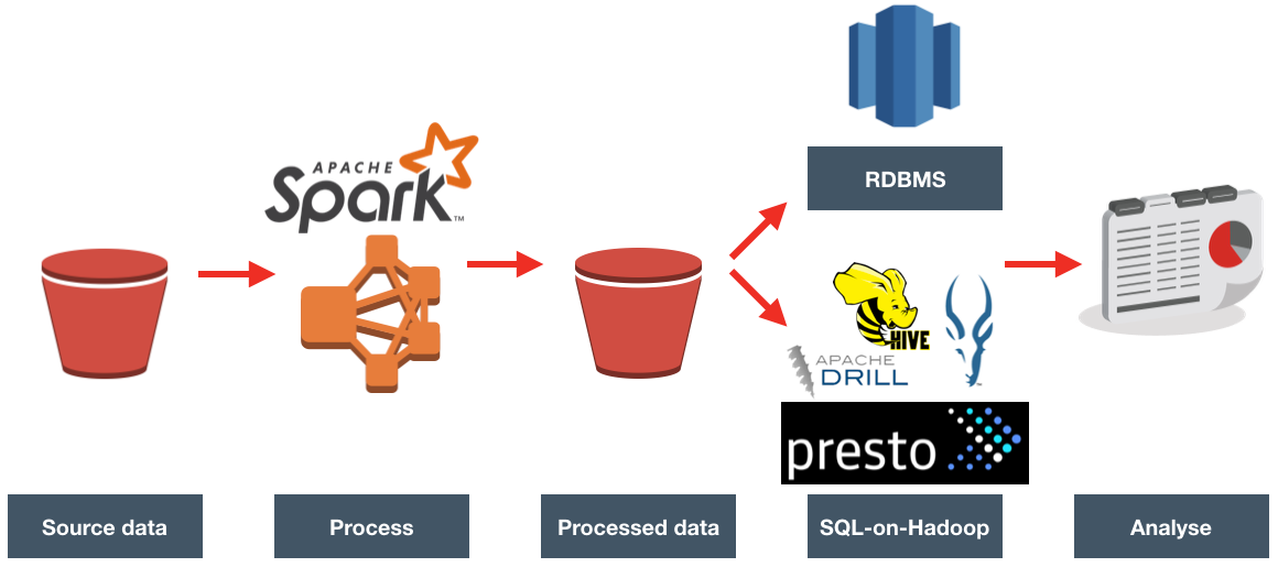
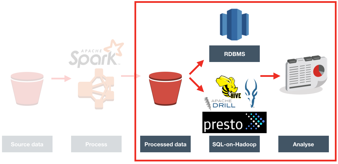
Big Data Discovery (BDD) is a great tool for exploring, transforming, and visualising data stored in your organisation’s Data Reservoir. I presented a workshop on it at a recent conference, and got an interesting question from the audience that I thought I’d explore further here. Currently the primary route for getting data into BDD requires that it be (i) in HDFS and (ii) have a Hive table defined on top of it. From there, BDD automagically ingests the Hive table, or the data_processing_CLI is manually called which prompts the BDD DGraph engine to go and sample (or read in full) the Hive dataset.
This is great, and works well where the dataset is vast (this is Big Data, after all) and needs the sampling that DGraph provides. It’s also simple enough for Hive tables that have already been defined, perhaps by another team. But – and this was the gist of the question that I got – what about where the Hive table doesn’t exist already? Because if it doesn’t, we now need to declare all the columns as well as choose the all-important SerDe in order to read the data.
SerDes are brilliant, in that they enable the application of a schema-on-read to data in many forms, but at the very early stages of a data project there are probably going to be lots of formats of data (such as TSV, CSV, JSON, as well as log files and so on) from varying sources. Choosing the relevant SerDe for each one, and making sure that BDD is also configured with the necessary jar, as well as manually listing each column to be defined in the table, adds overhead to the project. Wouldn’t it be nice if we could side-step this step somehow? In this article we’ll see how!
Importing Datasets through BDD Studio
Before we get into more fancy options, don’t forget that BDD itself offers the facility to upload CSV, TSV, and XLSX files, as well as connect to JDBC datasources. Data imported this way will be stored by BDD in a Hive table and ingested to DGraph.
This is great for smaller files held locally. But what about files on your BDD cluster, that are too large to upload from local machine, or in other formats – such as JSON?
Loading a CSV file
As we’ve just seen, CSV files can be imported to Hive/BDD directly through the GUI. But perhaps you’ve got a large CSV file sat local to BDD that you want to import? Or a folder full of varying CSV files that would be too time-consuming to upload through the GUI one-by-one?
For this we can use BDD Shell with the Python Pandas library, and I’m going to do so here through the excellent Jupyter Notebooks interface. You can read more about these here and details of how to configure them on BigDataLite 4.5 here. The great thing about notebooks, whether Jupyter or Zeppelin, is that I don’t need to write any more blog text here – I can simply embed the notebook inline and it is self-documenting:
Note that at end of this we call data_processing_CLI to automatically bring the new table into BDD’s DGraph engine for use in BDD Studio. If you’ve got BDD configured to automagically add new Hive tables, or you don’t want to run this step, you can just comment it out.
Loading simple JSON data
Whilst CSV files are tabular by definition, JSON records can contain nested objects (recursively), as well as arrays. Let’s look at an example of using SparkSQL to import a simple flat JSON file, before then considering how we handle nested and array formats. Note that SparkSQL can read datasets from both local (file://) storage as well as HDFS (hdfs://):
What’s been great so far, whether loading CSV, XLS, or simple JSON, is that we’ve not had to list out column names. All that needs modifying in the scripts above to import a different file with a different set of columns is to change the filename and the target tablename. Now we’re going to look at an example of a JSON file with nested objects – which is very common in JSON – and we’re going to have to roll our sleeves up a tad and start hardcoding some schema details.
First up, we import the JSON to a SparkSQL dataframe as before (although this time I’m loading it from HDFS, but local works too):
Here we use the LATERAL VIEW syntax, with the optional OUTER operator since not all tweets have these additional entities, and we want to make sure we show all tweets including those that don’t have these entities. Here’s the SQL formatted for reading:
SELECT id,
created_at,
user.screen_name,
text as tweet_text,
hashtag.text as hashtag,
user_mentions.screen_name as mentioned_user
from twitter
LATERAL VIEW OUTER explode(entities.user_mentions) user_mentionsTable as user_mentions
LATERAL VIEW OUTER explode(entities.hashtags) hashtagsTable AS hashtag
You can use these SQL queries both for simply flattening JSON, as above, or for building summary tables, such as this one showing the most common hashtags in the dataset:
sqlContext.sql("SELECT hashtag.text,count(*) as inst_count from twitter  LATERAL VIEW OUTER explode(entities.hashtags) hashtagsTable AS hashtag GROUP BY hashtag.text order by inst_count desc").show(4)

+-----------+----------+
|       text|inst_count|
+-----------+----------+
|     Hadoop|       165|
|     Oracle|       151|
|        job|       128|
|    BigData|       112|
You can find the full Jupyter Notebook with all these nested/array JSON examples here:
You may decide after looking at this that you’d rather just go back to Hive and SerDes, and as is frequently the case in ‘data wrangling’ there’s multiple ways to achieve the same end. The route you take comes down to personal preference and familiarity with the toolsets. In this particular case I’d still go for SparkSQL for the initial exploration as it’s quicker to ‘poke around’ the dataset than with defining and re-defining Hive tables — YMMV. A final point to consider before we dig in is that SparkSQL importing JSON and saving back to HDFS/Hive is a static process, and if your underlying data is changing (e.g. streaming to HDFS from Flume) then you would probably want a Hive table over the HDFS file so that it is live when queried.
Loading an Excel workbook with many sheets
This was the use-case that led me to researching programmatic import of datasets in the first place. I was doing some work with a dataset of road traffic accident data, which included a single XLS file with over 30 sheets, each a lookup table for a separate set of dimension attributes. Importing each sheet one by one through the BDD GUI was tedious, and being a lazy geek, I looked to automate it.
Using Pandas read_excel function and a smidge of Python to loop through each sheet it was easily done. You can see the full notebook here:
Oracle’s Big Data Discovery encompasses a good amount of exploration, transformation, and visualisation capabilities for datasets residing in your organisation’s data reservoir. Even with this though, there may come a time when your data scientists want to unleash their R magic on those same datasets. Perhaps the data domain expert has used BDD to enrich and cleanse the data, and now it’s ready for some statistical analysis? Maybe you’d like to use R’s excellent forecast package to predict the next six months of a KPI from the BDD dataset? And not only predict it, but write it back into the dataset for subsequent use in BDD? This is possible using BDD Shell and rpy2. It enables advanced analysis and manipulation of datasets already in BDD. These modified datasets can then be pushed back into Hive and then BDD.
BDD Shell provides a native Python environment, and you may opt to use the pandas library to work with BDD datasets as detailed here. In other cases you may simply prefer working with R, or have a particular library in mind that only R offers natively. In this article we’ll see how to do that. The “secret sauce” is rpy2 which enables the native use of R code within a python-kernel Jupyter Notebook.
As with previous articles I’m using a Jupyter Notebook as my environment. I’ll walk through the code here, and finish with a copy of the notebook so you can see the full process.
First we’ll see how you can use R in Jupyter Notebooks running a python kernel, and then expand out to integrate with BDD too. You can view and download the first notebook here.
Import the RPY2 environment so that we can call R from Jupyter
import readline is necessary to workaround the error: /u01/anaconda2/lib/libreadline.so.6: undefined symbol: PC
import readline
%load_ext rpy2.ipython
Example usage
Single inline command, prefixed with %R
%R X=c(1,4,5,7); sd(X); mean(X)
array([ 4.25])
R code block, marked by %%R
%%R
Y = c(2,4,3,9)
summary(lm(Y~X))
Call:
lm(formula = Y ~ X)

Residuals:
    1     2     3     4
 0.88 -0.24 -2.28  1.64

Coefficients:
            Estimate Std. Error t value Pr(>|t|)
(Intercept)   0.0800     2.3000   0.035    0.975
X             1.0400     0.4822   2.157    0.164

Residual standard error: 2.088 on 2 degrees of freedom
Multiple R-squared:  0.6993,    Adjusted R-squared:  0.549
F-statistic: 4.651 on 1 and 2 DF,  p-value: 0.1638
Working with BDD Datasets from R in Jupyter Notebooks
Now that we’ve seen calling R in Jupyter Notebooks, let’s see how to use it with BDD in order to access datasets. The first step is to instantiate the BDD Shell so that you can access the datasets in BDD, and then to set up the R environment using rpy2
Note that there is a lot of passing of the same dataframe into different memory structures here – from BDD dataset context to Spark to Pandas, and that’s before we’ve even hit R. It’s fine for ad-hoc wrangling but might start to be painful with very large datasets.
Now we use the rpy2 integration with Jupyter Notebooks and invoke R parsing of the cell’s contents, using the %%R syntax. Optionally, we can pass across variables with the -i parameter, which we’re doing here. Then we assign the dataframe to an R-notation variable (optional, but stylistically nice to do), and then use R’s summary function to show a summary of each attribute:
%%R -i pandas_df
R.df <- pandas_df
summary(R.df)
vendorid     tpep_pickup_datetime tpep_dropoff_datetime passenger_count
 Min.   :1.000   Min.   :1.420e+12    Min.   :1.420e+12     Min.   :0.000
 1st Qu.:1.000   1st Qu.:1.427e+12    1st Qu.:1.427e+12     1st Qu.:1.000
 Median :2.000   Median :1.435e+12    Median :1.435e+12     Median :1.000
 Mean   :1.525   Mean   :1.435e+12    Mean   :1.435e+12     Mean   :1.679
 3rd Qu.:2.000   3rd Qu.:1.443e+12    3rd Qu.:1.443e+12     3rd Qu.:2.000
 Max.   :2.000   Max.   :1.452e+12    Max.   :1.452e+12     Max.   :9.000
 NA's   :12      NA's   :12           NA's   :12            NA's   :12
 trip_distance      pickup_longitude  pickup_latitude    ratecodeid
 Min.   :    0.00   Min.   :-121.93   Min.   :-58.43   Min.   : 1.000
 1st Qu.:    1.00   1st Qu.: -73.99   1st Qu.: 40.74   1st Qu.: 1.000
 Median :    1.71   Median : -73.98   Median : 40.75   Median : 1.000
 Mean   :    3.04   Mean   : -72.80   Mean   : 40.10   Mean   : 1.041
 3rd Qu.:    3.20   3rd Qu.: -73.97   3rd Qu.: 40.77   3rd Qu.: 1.000
 Max.   :67468.40   Max.   : 133.82   Max.   : 62.77   Max.   :99.000
 NA's   :12         NA's   :12        NA's   :12       NA's   :12
 store_and_fwd_flag dropoff_longitude dropoff_latitude  payment_type
 N   :992336        Min.   :-121.93   Min.   : 0.00    Min.   :1.00
 None:    12        1st Qu.: -73.99   1st Qu.:40.73    1st Qu.:1.00
 Y   :  8218        Median : -73.98   Median :40.75    Median :1.00
                    Mean   : -72.85   Mean   :40.13    Mean   :1.38
                    3rd Qu.: -73.96   3rd Qu.:40.77    3rd Qu.:2.00
                    Max.   :   0.00   Max.   :44.56    Max.   :5.00
                    NA's   :12        NA's   :12       NA's   :12
  fare_amount          extra            mta_tax          tip_amount
 Min.   :-170.00   Min.   :-1.0000   Min.   :-1.7000   Min.   :  0.000
 1st Qu.:   6.50   1st Qu.: 0.0000   1st Qu.: 0.5000   1st Qu.:  0.000
 Median :   9.50   Median : 0.0000   Median : 0.5000   Median :  1.160
 Mean   :  12.89   Mean   : 0.3141   Mean   : 0.4977   Mean   :  1.699
 3rd Qu.:  14.50   3rd Qu.: 0.5000   3rd Qu.: 0.5000   3rd Qu.:  2.300
 Max.   : 750.00   Max.   :49.6000   Max.   :52.7500   Max.   :360.000
 NA's   :12        NA's   :12        NA's   :12        NA's   :12
  tolls_amount      improvement_surcharge  total_amount       PRIMARY_KEY
 Min.   : -5.5400   Min.   :-0.3000       Min.   :-170.80   0-0-0   :      1
 1st Qu.:  0.0000   1st Qu.: 0.3000       1st Qu.:   8.75   0-0-1   :      1
 Median :  0.0000   Median : 0.3000       Median :  11.80   0-0-10  :      1
 Mean   :  0.3072   Mean   : 0.2983       Mean   :  16.01   0-0-100 :      1
 3rd Qu.:  0.0000   3rd Qu.: 0.3000       3rd Qu.:  17.80   0-0-1000:      1
 Max.   :503.0500   Max.   : 0.3000       Max.   : 760.05   0-0-1001:      1
 NA's   :12         NA's   :12            NA's   :12        (Other) :1000560
We can use native R code and R libraries including the excellent dplyr to lightly wrangle and then chart the data:
Oracle Stream Analytics (OSA) is a graphical tool that provides “Business Insight into Fast Data”. In layman terms, that translates into an intuitive web-based interface for exploring, analysing, and manipulating streaming data sources in realtime. These sources can include REST, JMS queues, as well as Kafka. The inclusion of Kafka opens OSA up to integration with many new-build data pipelines that use this as a backbone technology.
Previously known as Oracle Stream Explorer, it is part of the SOA component of Fusion Middleware (just as OBIEE and ODI are part of FMW too). In a recent blog it was positioned as “[…] part of Oracle Data Integration And Governance Platform.”. Its Big Data credentials include support for Kafka as source and target, as well as the option to execute across multiple nodes for scaling performance and capacity using Spark.
I’ve been exploring OSA from the comfort of my own Mac, courtesy of Docker and a Docker image for OSA created by Guido Schmutz. The benefits of Docker are many and covered elsewhere, but what I loved about it in this instance was that I didn’t have to download a VM that was 10s of GB. Nor did I have to spend time learning how to install OSA from scratch, which whilst interesting wasn’t a priority compared to just trying to tool out and seeing what it could do. [Update] it turns out that installation is a piece of cake, and the download is less than 1Gb … but in general the principle still stands – Docker is a great way to get up and running quickly with something
In this article we’ll take OSA for a spin, looking at some of the functionality and terminology, and then real examples of use with live Twitter data.
To start with, we sign in to Oracle Stream Analytics:
From here, click on the Catalog link, where a list of all the resources are listed. Some of these resource types include:
Streams – definitions of sources of data such as Kafka, JMS, and a dummy data generator (event generator)
Connections – Servers etc from which Streams are defined
Explorations – front-end for seeing contents of Streams in realtime, as well as applying light transformations
Targets – destination for transformed streams
Viewing Realtime Twitter Data with OSA
The first example I’ll show is the canonical big data/streaming example everywhere – Twitter. Twitter is even built into OSA as a Stream source. If you go to https://dev.twitter.com you can get yourself a set of credentials enabling you to query the live Twitter firehose for given hashtags or users.
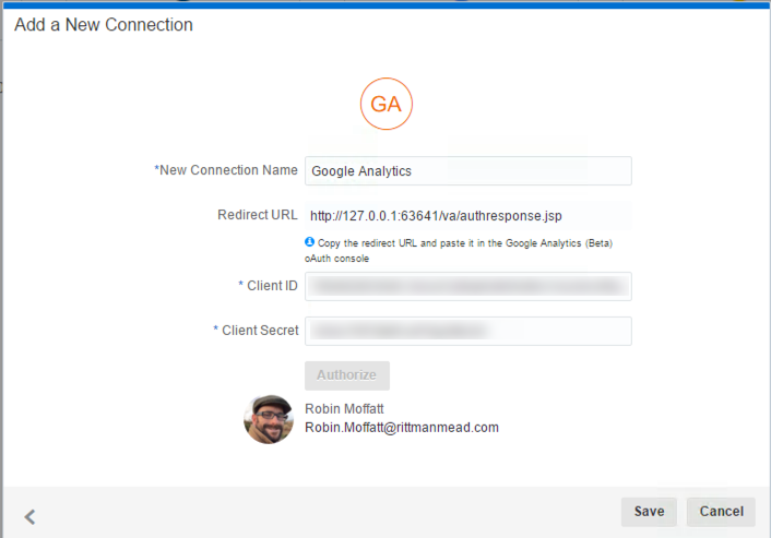
With my twitter dev credentials, I create a new Connection in OSA:
Now we have an entry in the Catalog, for the Twitter connection:
from which we can create a Stream, using the connection and a set of hashtags or users for whom we want to stream tweets:
The Shape is basically the schema or data model that is applied for the stream. There is one built-in for Twitter, which we’ll use here:
When you click Save, if you get an error Unable to deploy OEP application then check the OSA log file for errors such as unable to reach Twitter, or invalid credentials.
Assuming the Stream is created successfully you are then prompted to create an Exploration from where you can see the Stream in realtime:
Explorations can have multiple stream sources, and be used to transform the contents, which we’ll see later. For now, after clicking Create, we get our Exploration window, which shows the contents of the stream in realtime:
At the bottom of the screen there’s the option to plot one or more charts showing the value of any numeric values in the stream, as can be seen in the animation above.
I’ll leave this example here for now, but finish by using the Publish option from the Actions menu, which makes it available as a source for subsequent analyses.
Adding Lookup Data to Streams
Let’s look now at some more of the options available for transforming and ‘wrangling’ streaming data with OSA. Here I’m going to show how two streams can be joined together (but not crossed) based on a common field, and the resulting stream used as the input for a subsequent process. The data is simulated, using a CSV file (read by OSA on a loop) and OSA’s Event Generator.
From the Catalog page I create a new Stream, using Event Generator as the Type:
On the second page of the setup I define how frequently I want the dummy events to be generated, and the specification for the dummy data:
The last bit of setup for the stream is to define the Shape, which is the schema of data that I’d like generated:
The Exploration for this stream shows the dummy data:
The second stream is going to be sourced from a very simple key/value CSV file:
The stream type is CSV, and I can configure how often OSA reads from it, as well as telling OSA to loop back to the beginning when it’s read to the end, thus simulating a proper stream. The ‘shape’ is picked up automatically from the file, based on the first row (headers) and then inferred data types:
The Exploration for the stream shows the five values repeatedly streamed through (since I ticked the box to ‘loop’ the CSV file in the stream):
Back on the Catalog page I’m going to create a new Exploration, but this time based on a Pattern. Patterns are pre-built templates for stream manipulation and processing. Here we’ll use the pattern for a “left outer join” between streams.
The Pattern has a set of pre-defined fields that need to be supplied, including the stream names and the common field with which to join them. Note also that I’ve increased the Window Range. This is necessary so that a greater range of CSV stream events are used for the lookup. If the Range is left at the default of 1 second then only events from both streams occurring in the same second that match on attr_id would be matched. Unless both streams happen to be in sync on the same attr_id from the outset then this isn’t going to happen that often, and certainly wouldn’t in a real-life data stream.
So now we have the two joined streams:
Within an Exploration it is possible to do light transformation work. By right-clicking on a column you can rename or remove it, which I’ve done here for the duplicated attr_id (duplicated since it appears in both streams), as well as renamed the attr_value:
Daisy-Chaining, Targets, and Topology
Once an Exploration is Published it can be used as the Source for subsequent Explorations, enabling you to map out a pipeline based on multiple source streams and transformations. Here we’re taking the exploration created just above that joined the two streams together, and using the output as the source for a new Exploration:
Since the Exploration is based on a previous one, the same stream data is available, but with the joins and transformations already applied
From here another transformation could be applied, such as replacing the value of one column conditionally based on that of another
Whilst OSA enables rapid analysis and transformation of inbound streams, it also lets you stream the transformed results outside of OSA, to a Target as we saw in the Kafka example above. As well as Kafka other technologies are supported as targets, including a REST endpoint, or a simple CSV file.
With a target configured, as well as an Exploration based on the output of another, the Topology comes in handy for visualising the flow of data. You can access this from the Topology icon in an Exploration page, or from the dropdown menu on the Catalog page against a given object
In the next post I will look at how Oracle Stream Analytics can be used to analyse, enrich, and publish data to and from Kafka. Stay tuned!
In my previous post I looked the latest release of Oracle Stream Analytics (OSA), and saw how it provided a graphical interface to “Fast Data”. Users can analyse streaming data as it arrives based on conditions and rules. They can also transform the stream data, publishing it back out as a stream in its own right. In this article we’ll see how OSA can be used with Kafka.
Kafka is one of the foremost streaming technologies nowadays, for very good reasons. It is highly scalable and flexible, supporting multiple concurrent consumers. Oracle Streaming Analytics supports Kafka as both a source and target. To set up an inbound stream from Kafka, first we define the Connection:
Once the Connection is defined, we can create a Stream for a given Kafka topic:
If you get an error at this point of Unable to deploy OEP application then check the OSA log – it could be a connectivity issue to Zookeeper.
Exception in thread "SpringOsgiExtenderThread-286" org.springframework.beans.FatalBeanException:
Error in context lifecycle initialization; nested exception is com.bea.wlevs.ede.api.EventProcessingException:
org.I0Itec.zkclient.exception.ZkTimeoutException:
Unable to connect to zookeeper server within timeout: 6000
Assuming that the Stream is saved with no errors, you can then create an Exploration based on the stream and all being well, the live tweets are soon shown. Unlike the example at the top of this article, these tweets are coming in via Kafka, rather than the built-in OSA Twitter Stream. This is partly to demonstrate the Kafka capabilities, but also because the built-in OSA Twitter Stream only includes a subset of the available twitter data fields.
Avro? Nope.
Data in Kafka can be serialised in many formats, including Avro – which OSA doesn’t seem to like. No error is thrown to the GUI but the exploration remains blank.
Looking in the OSA log file there’s a whole lot of errors recorded similar to this:
line 1:0 no viable alternative at character '?'
line 1:1 no viable alternative at character '?'
line 1:2 no viable alternative at character '?'
line 1:3 no viable alternative at character '?'
line 1:4 no viable alternative at character '?'
line 1:5 no viable alternative at character '?'
line 1:6 no viable alternative at character '?'
line 1:7 no viable alternative at character '?'
line 1:8 no viable alternative at character ''
JSON? Kinda.
One of the challenges that I found working with OSA was defining the “Shape” (data model) of the inbound stream data. JSON is a format used widely as a technology-agnostic data interchange format, including for the twitter data that I was working with. You can see a sample record here. One of the powerful features of JSON is its ability to nest objects in a record, as well as create arrays of them. You can read more about this detail in a recent article I wrote here. Unfortunately it seems that OSA does not support flattening out JSON, meaning that only elements in the root of the model are accessible. For twitter, that means we can see the text, and who it was in reply to, but not the user who tweeted it, since the latter is a nested element (along with many other fields, including hashtags which are also an array):
So what to do if the inbound streaming data is in nested-JSON format? It seems to me the only option is to pre-process it to flatten it. There are a variety of tools that could be used here – in the first instance I’d generally reach for Logstash, it being the one I’m most familiar with. To get an idea of the schema of a JSON record you can use jsonschema.net. Funnily enough when I was researching this blog post I came across the exact same problem on a forum posted by … me! Early last year I was working with the same dataset, and had the same issue with embedded arrays. The way to do it in Logstash is with a bit of Ruby code to flatten the arrays, and a standard mutate to bring nested objects up to the root level. Sample code:
You can find the full Logstash code on gist here. With this logstash code running I set up a new OSA Stream pointing to the new Kafka topic that Logstash was writing, and added the flattened fields to the Shape:
We can then see in the Exploration the fields that we wanted to get at – user name, hashtags, and so on:
Other Shape Gotchas
One of the fields in Twitter data is ‘source’ – which unfortunately is a reserved identifier in the CQL language that OSA uses behind the scenes.
Caused By: org.springframework.beans.FatalBeanException: Exception initializing channel; nested exception is com.bea.wlevs.ede.api.ConfigurationException: Event type [sx-10-16-Kafka_Technology_Tweets_JSON-1] of channel [channel] uses invalid or reserved CQL identifier = , source
It’s not clear how to define a shape in which the source data field is named after a reserved identifier.
Further Exploration of Twitter Streams with OSA
Using the flattened Twitter stream coming via Kafka that I demonstrated above, let’s now look at more OSA functionality.
Depending on the source of your data stream, and your purpose for analysing it, you may well want to filter out certain content. This can be done from the Exploration screen:
The Business Rules section of the Exploration enables you to define rules about the data and set field values based on it. This can be static values, or expressions based on data in the stream. There doens’t seem to be a way to add arbitrary fields via this, so I amended the Stream Shape to include a ‘spare’ field that I then populated:
Kafka Stream Transformation with OSA
Here we’ll see how OSA can be used to ingest one Kafka topic, apply a transformation, and stream it to another Kafka topic.
The OSA exploration screen offers a basic aggregation (‘summary’) function, here showing the number of tweets per language:
Using the Windows icon to the right of the Sources box the time window can be defined, along with the refresh frequency:
This means that the count of tweets per language will be calculated looking at the data for the past 30 seconds, and this will be evaluated every five seconds. More complex functionality such as pivoting on the group-by column (so as to be able to chart out the number of tweets per language as separate metrics) doesn’t seem to be present in this release; arguably this is moving over into per analytics territory such as would be found in Oracle’s Big Data Discovery.
Taking the summarised stream (count of tweets, by language) I first Publish the exploration, making it available for use as the input to a subsequent exploration. Then from the Catalog page select a Pattern, which I’m going to use to build a stream showing the most common languages in the past five seconds. With the Top N pattern you specify the event stream (in this case, the summarised stream that I built above), and the metric by which to order the events which here is the count of tweets per language.
For completeness, I’m going to stream the output of this pattern exploration back to a Kafka topic
Note that I’ve defined a new Shape here based on the columns in the pattern. In the pattern itself I renamed the COUNT column to a clearer one (tweet_count_5_sec). Renaming it wasn’t strictly necessary since it’s possible to define the field/shape mapping when you configure the Target:
For the target to take effect, I publish the pattern exploration, and then using kafka-console-consumer can see the topic being populated in realtime by OSA:
Being able to apply transformations to streams in realtime like this and stream the results is pretty useful. There are some limitations to the capabilities of OSA through the front end GUI. For example, support for nested json, and integration with the Kafka Schema Registry to automatically derive Shapes for inbound topics would both be great. Lower-level, the option to specify the consumer group id, as well as the start point for consumption (beginning of topic, or streaming at the end) are both things that would probably be necessary sooner or later using OSA for full-blown development.
OSA and Spatial
One of the Patterns that OSA provides is a Spatial one, which can be used to analyse source data that includes geo-location data. This could be to simply plot the occurrence of the data point (as we’ll see shortly) on a map. It can also be used in a more sophisticated manner, to track a given entity’s movements on a map. An example of this could be a fleet of trucks reporting their position back at regular intervals. Areas on a map can be defined and conditions triggered as the entity enters or leaves the area. For now though, we’ll keep it simple. Using the flattened Twitter stream from Kafka that I produced from Logstash above, I’m going to plot Tweets in realtime on a map, along with a very simplistic tagging of the broad area in which they came from.
In my source Kafka topic I have two fields, latitude and longitude. I expose these as part of the ‘flattening’ of the JSON in this logstash script, since by default they’re nested within the coordinates field and as an array too. When defining the Stream’s Shape make sure you define the datatype correctly (Double) – OSA is not very forgiving of stupidity and I spent a frustrating time trying to work out why “-80.1422195” was coming through as zero – obviously defined as an Integer this was never going to work!
Not entirely necessary, but useful for debug purposes, I setup an exploration based on the flattened Twitter stream, with a filter to only include tweets that had geo-location data in them. This way I knew what tweets I should expect to be seeing in the next step. One of the things that I have found with OSA is that it has a tendency to fail silently; instead of throwing errors you’ll just not get any data. By setting up the filter exploration I could at least debug things a bit more easily.
After this I created a new object, a Map. A Map object defines a set of named areas, which could be sourced from a database table, or drawn manually – which is what I did here by setting the Map Type to ‘None (Create Manually)’. One thing to note about the maps is that they’re sourced online (openstreetmap.org) so you’ll need an internet connection to do this. Once the Map is open, click the Polygon Tool icon and click-drag a shape around the area that you want to “geo-fence”. Each area is given a name, and this is what is used in the streaming data to label the event’s geographical area.
Having got our source data stream with geo-data in, and a Map on which to plot it and analyse the location of each event, we now use the Spatial General pattern to create an Exploration. The topology looks like this:
The fields in the Spatial General pattern are all pretty obvious. Object key is the field to use to track the same entity across multiple events, if you want to use the enter/exit/stay statuses. For tweets we just use ‘Enter’, but for people or vehicles, for example, you might get multiple status reports and want to track them on a map. For example, when a person is near a point of interest that you’re tracking, or a vehicle has remained in a set area for too long.
If you let the Exploration now run, depending on the rate of event ingest, you’ll sooner or later see points appearing on the map and event details underneath. The “status” column is populated (blank if the event is outside of the defined geo-fences), as is the “Place”, based on the geo-fence names that you defined.
Summary
I can see OSA being used in two ways. The first as an ‘endpoint’ for streams with users taking actions based on the data, with some of the use cases listed here. The second is for prototyping transformations and analyses on streams prior to productionising them. The visual interface and immediacy of feedback on transformations applied means that users can quickly understand what further processing they may want to apply to the stream using actual streaming data to inform this.
This latter concept – that of prototyping – is similar to that which we see with another of Oracle’s products, Big Data Discovery. With BDD users can analyse data in the organisation’s data reservoir, as well as apply transformations to it (read more). Just as BDD doesn’t replace OBIEE or Visual Analyzer but enables users to understand how they do want to model the data in these tools, OSA wouldn’t replace “production grade” integration done by Oracle Data Integrator. What it would do is allow users to get a clearer idea of the transformations they would want performed in it.
OSA’s user interface is easy to use and intuitive, and this is definitely a tool that you would put in front of technically minded business users. There are limitations to what can be achieved technically through the web GUI alone and something like Oracle Data Integrator (ODI) would still be a more appropriate fit for complex streaming work. At Oracle Open World last year it was announced (slides) that a beta would be starting for ODI using Spark Streaming for ETL and stream processing, so it’ll be interesting to see this when it comes out.
Oracle release their "Critical Patch Update" (CPU) notices every quarter, bundling together details of vulnerabilities and associated patches across their entire product line. October's was released yesterday, with a few entries of note in the analytics & DI space.
Each vulnerability is given a unique identifier (CVE-xxxx-xxxx) and a score out of ten. The scoring uses a common industry-standard scale on the basis of how easy it is to exploit, and what is compromised (availability, data, etc). Ten is the worst, and I would crudely paraphrase it as generally meaning that someone can wander in, steal your data, change your data, and take your system offline. Lower than that and it might be that it requires extensive skills to exploit, or the impact be much lower.
A final point to note is that the security patches that are released are not available for old versions of the software. For example, if you're on OBIEE 11.1.1.6 or earlier, and it is affected by the vulnerability listed below (which I would assume it is), there is no security patch. So even if you don't want to update your version for the latest functionality, staying within support is an important thing to do and plan for. You can see the dates for OBIEE versions and when they go out of "Error Correction Support" here.
If you want more information on how Rittman Mead can help you plan, test, and carry out patching or upgrades, please do get in touch!
The vulnerabilities listed below are not a comprehensive view of an Oracle-based analytics/DI estate - things like the database itself, along with Web Logic Server, should also be checked. See the CPU itself for full details.
This vulnerability documents the potential that a developer could take the master repository schema credentials and use them to grant themselves SUPERVISOR access. Even using the secure wallet, the credentials are deobfuscated on the local machine and therefore a malicious developer could still access the credentials in theory.
To use Data Visualisation Desktop (DVD) with data from Google Analytics or Google Drive, you need to set up the necessary credentials on Google so that DVD can connect to it. You can see a YouTube of this process on this blog here.
Before starting, you need a piece of information from Oracle DVD that will be provided to Google during the setup. From DVD, create a new connection of type Google Analytics, and make a note of the the provided redirect URL:
Once you have this URL, you can go and set up the necessary configuration in Google. To do this, go to https://console.developers.google.com/ and sign in with the same Google credentials as have acces to Google Analytics.
Having created the project, we now need to make available the necessary APIs to it, after which we will create the credentials. Go to https://console.developers.google.com/apis/ and click on Analytics API
On the next screen, click Enable, which adds this API to the project.
If you want, at this point you can return to the API list and also add the Google Drive API by selecting and then Enabling it.
Now we will create the credentials required. Click on Credentials, and then on OAuth consent screen. Fill out the Product name field.
Click on Save, and then on the next page click on Create credentials and from the dropdown list OAuth client ID
Set the Application type to Web Application, give it a name, and then copy the URL given in the DVD New Connection window into the Authorised redirect URIs field.
Click Create, and then make a note of the provided client ID and client secret. Watch out for any spaces before or after the values (h/t @Nephentur). Keep these credentials safe as you would any password.
Go back to DVD and paste these credentials into the Create Connection screen, and click Authorise. When prompted, sign in to your Google Account.
Click on Save, and your connection is now created successfully!
With a connection to Google Analytics created, you can now analyse the data available from within it. You'll need to set the measure columns appropriately, as by default they're all taken by DVD to be dimensions.
I wrote recently about what Apache Drill is, and how to use it with OBIEE. In this post I wanted to demonstrate its great power in action for a requirement that came up recently. We wanted to analyse our blog traffic, broken down by blog author. Whilst we have Google Analytics to provide the traffic, it doesn't include the blog author. This is held within the blog platform, which is Ghost. The common field between the two datasets is the post "slug". From Ghost we could get a dump of the data in JSON format. We needed to find a quick way to analyse and extract from this JSON a list of post slugs and associated author.
One option would be to load the JSON into a RDBMS and process it from within there, running SQL queries to extract the data required. For a long-term large-scale solution, maybe this would be appropriate. But all we wanted to do here was query a single file, initially just as a one-off. Enter Apache Drill. Drill can run on a single laptop (or massively clustered, if you need it). It provides a SQL engine on top of various data sources, including text data on local or distributed file systems (such as HDFS).
You can use Drill to dive straight into the json:
0: jdbc:drill:zk=local> use dfs;
+-------+----------------------------------+
|  ok   |             summary              |
+-------+----------------------------------+
| true  | Default schema changed to [dfs]  |
+-------+----------------------------------+
1 row selected (0.076 seconds)
0: jdbc:drill:zk=local> select * from `/Users/rmoff/Downloads/rittman-mead.ghost.2016-11-01.json` limit 1;
+----+
| db |
+----+
| [{"meta":{"exported_on":1478002781679,"version":"009"},"data":{"permissions":[{"id":1,"uuid":"3b24011e-4ad5-42ed-8087-28688af7d362","name":"Export database","object_type":"db","action_type":"exportContent","created_at":"2016-05-23T11:24:47.000Z","created_by":1,"updated_at":"2016-05-23T11:24:47.000Z","updated_by":1},{"id":2,"uuid":"55b92b4a-9db5-4c7f-8fba-8065c1b4b7d8","name":"Import database","object_type":"db","action_type":"importContent","created_at":"2016-05-23T11:24:47.000Z","created_by":1,"updated_at":"2016-05-23T11:24:47.000Z","updated_by":1},{"id":3,"uuid":"df98f338-5d8c-4683-8ac7-fa94dd43d2f1","name":"Delete all content","object_type":"db","action_type":"deleteAllContent","created_at":"2016-05-23T11:24:47.000Z","created_by":1,"updated_at":"2016-05-23T11:24:47.000Z","updated_by":1},{"id":4,"uuid":"a3b8c5c7-7d78-442f-860b-1cea139e1dfc","name":"Send mail","object_type":"mail","action_
But from this we can see the JSON object is a single column db of array type. Let's take a brief detour into one of my favourite commandline tools - jq. This let's you format, filter, and extract values from JSON. Here we can use it to get an idea of how the data's structured. We can do this in Drill, but jq gives us a headstart:
We can see that under the db array are two elements; meta and data. Let's take meta as a simple example to expose through Drill, and then build from there into the user data that we're actually after.
Since the root data element (db) is an array, we need to FLATTEN it:
0: jdbc:drill:zk=local> with db as (select flatten(db) from `/Users/rmoff/Downloads/rittman-mead.ghost.2016-11-01.json`) select db.meta from db limit 1;
Nov 01, 2016 2:18:31 PM org.apache.calcite.sql.validate.SqlValidatorException <init>
SEVERE: org.apache.calcite.sql.validate.SqlValidatorException: Column 'meta' not found in table 'db'
Nov 01, 2016 2:18:31 PM org.apache.calcite.runtime.CalciteException <init>
SEVERE: org.apache.calcite.runtime.CalciteContextException: From line 1, column 108 to line 1, column 111: Column 'meta' not found in table 'db'
Error: VALIDATION ERROR: From line 1, column 108 to line 1, column 111: Column 'meta' not found in table 'db'

SQL Query null

[Error Id: 9cb4aa98-d522-42bb-bd69-43bc3101b40e on 192.168.10.72:31010] (state=,code=0)
This didn't work, because if you look closely at the above FLATTEN, the resulting column is called EXPR$0, so we need to alias it in order to be able to reference it:
0: jdbc:drill:zk=local> select flatten(db) as db from `/Users/rmoff/Downloads/rittman-mead.ghost.2016-11-01.json`;
+----+
| db |
+----+
| {"meta":{"exported_on":1478002781679,"version":"009"},"data":{"permissions":[{"id":1,"uuid":"3b24011e-4ad5-42ed-8087-28688af7d362","name":"Export database","object_type":"db","action_type":"exportConten
Having done this, I'll put the FLATTEN query as a subquery using the WITH syntax, and from that SELECT just the meta elements:
0: jdbc:drill:zk=local> with ghost as (select flatten(db) as db from `/Users/rmoff/Downloads/rittman-mead.ghost.2016-11-01.json`) select ghost.db.meta from ghost limit 1;
+------------------------------------------------+
|                     EXPR$0                     |
+------------------------------------------------+
| {"exported_on":1478002781679,"version":"009"}  |
+------------------------------------------------+
1 row selected (0.317 seconds)
Note that the column is EXPR$0 because we've not defined a name for it. Let's fix that:
0: jdbc:drill:zk=local> with ghost as (select flatten(db) as db from `/Users/rmoff/Downloads/rittman-mead.ghost.2016-11-01.json`) select ghost.db.meta as meta from ghost limit 1;
+------------------------------------------------+
|                      meta                      |
+------------------------------------------------+
| {"exported_on":1478002781679,"version":"009"}  |
+------------------------------------------------+
1 row selected (0.323 seconds)
0: jdbc:drill:zk=local>
Why's that matter? Because it means that we can continue to select elements from within it.
We could continue to nest the queries, but it gets messy to read, and complex to debug any issues. Let's take this meta element as a base one from which we want to query, and define it as a VIEW:
0: jdbc:drill:zk=local> create or replace view dfs.tmp.ghost_meta as with ghost as (select flatten(db) as db from `/Users/rmoff/Downloads/rittman-mead.ghost.2016-11-01.json`) select ghost.db.meta as meta from ghost;
+-------+-------------------------------------------------------------+
|  ok   |                           summary                           |
+-------+-------------------------------------------------------------+
| true  | View 'ghost_meta' created successfully in 'dfs.tmp' schema  |
+-------+-------------------------------------------------------------+
1 row selected (0.123 seconds)
Now we can select from the view:
0: jdbc:drill:zk=local> select m.meta.exported_on as exported_on, m.meta.version as version from dfs.tmp.ghost_meta m;
+----------------+----------+
|  exported_on   | version  |
+----------------+----------+
| 1478002781679  | 009      |
+----------------+----------+
1 row selected (0.337 seconds)
Remember that when you're selected nested elements you must alias the object that you're selecting from. If you don't, then Drill assumes that the first element in the column name (for example, meta.exported_on) is the table name (meta), and you'll get an error:
Error: VALIDATION ERROR: From line 1, column 8 to line 1, column 11: Table 'meta' not found
So having understood how to isolate and query the meta element in the JSON, let's progress onto what we're actually after - the name of the author of each post, and associated 'slug'.
Using jq again we can see the structure of the JSON file, with the code taken from here:
So Posts data is under the data.posts element, and from manually poking around we can see that user data is under data.users element.
Back to Drill, we'll create views based on the same pattern as we used for meta above; flattening the array and naming the column:
use dfs.tmp;
create or replace view ghost_posts as select flatten(ghost.db.data.posts) post from ghost;
create or replace view ghost_users as select flatten(ghost.db.data.users) `user` from ghost;
The ghost view is the one created above, in the dfs.tmp schema. With these two views created, we can select values from each:
0: jdbc:drill:zk=local> select u.`user`.id,u.`user`.name from ghost_users u where u.`user`.name = 'Robin Moffatt';
+---------+----------------+
| EXPR$0  |     EXPR$1     |
+---------+----------------+
| 15      | Robin Moffatt  |
+---------+----------------+
1 row selected (0.37 seconds)

0: jdbc:drill:zk=local> select p.post.title,p.post.slug,p.post.author_id from ghost_posts p where p.post.title like '%Drill';
+----------------------------------+----------------------------------+---------+
|              EXPR$0              |              EXPR$1              | EXPR$2  |
+----------------------------------+----------------------------------+---------+
| An Introduction to Apache Drill  | an-introduction-to-apache-drill  | 15      |
+----------------------------------+----------------------------------+---------+
1 row selected (0.385 seconds)
and join them:
0: jdbc:drill:zk=local> select p.post.slug as post_slug,u.`user`.name as author from ghost_posts p inner join ghost_users u on p.post.author_id = u.`user`.id where u.`user`.name like 'Robin%' and p.post.status='published' order by p.post.created_at desc limit 5;
+------------------------------------------------------------------------------------+----------------+
|                                     post_slug                                      |     author     |
+------------------------------------------------------------------------------------+----------------+
| connecting-oracle-data-visualization-desktop-to-google-analytics-and-google-drive  | Robin Moffatt  |
| obiee-and-odi-security-updates-october-2016                                        | Robin Moffatt  |
| otn-appreciation-day-obiees-bi-server                                              | Robin Moffatt  |
| poug                                                                               | Robin Moffatt  |
| all-you-ever-wanted-to-know-about-obiee-performance-but-were-too-afraid-to-ask     | Robin Moffatt  |
+------------------------------------------------------------------------------------+----------------+
5 rows selected (1.06 seconds)
This is pretty cool. From a 32MB single-row JSON file:
to being able to query it with standard SQL like this:
all with a single tool that can run on a laptop or desktop, and supports ODBC and JDBC for use with your favourite BI tools. For data exploration and understanding new datasets, Apache Drill really does rock!
We have a strong innovation spirit at Rittman Mead, with all staff encouraged to use technology to its best advantage in order to do things with the software that haven't been done before. Some of these projects may may be 'scratching the itch' of a repeated manual task that should be automated. Others use technology to extend the capabilities of the tools or write new ones to fill gaps that have been identified.
At Rittman Mead we pride ourselves in our sharing of knowledge with the BI/DI community, both 'offline' at conferences and online through our blog. Today we are excited to extend this further, with the release over the next few days and weeks into open-source of some key code projects: -
insights - a javascript API/framework for building a new frontend for OBIEE, building on the OBIEE web service interface. Read more here.
vpp - "Visual Plugin Pack" - enable OBIEE Answers report builders to use and configure JS visualisations through native OBIEE user interface - no coding required! Read more here.
We're very excited about opening up these projects to the community, and would be delighted to see forks and pull-requests as people build and expand on them. It should go without saying, but these are contributed 'as is'; any bugs and problems you find we will happily receive a pull request for :-)
If you would like help implementing and extending these for your own project, we would be delighted to offer services in doing so - just get in touch to find out more.
OBIEE provides Usage Tracking as part of the core product functionality. It writes directly to a database table every Logical Query that hits the BI Server, including details of who ran it, when, and information about how it executed including for how long, how many rows, and so on. This in itself is a veritable goldmine of information about your OBIEE system. All OBIEE deployments should have Usage Tracking enabled, for supporting performance analysis, capacity planning, catalog rationalisation, and more.
What Usage Tracking doesn't track is interactions between the end user and the Presentation Services component. Presentation Services sits between the end user and the BI Server from where the actual queries get executed. This means that until a user executes an analysis, there's no record of their actions in Usage Tracking. There is this audit data available, but you have to manually enable and collect it, which can be tricky. This is where Enhanced Usage Tracking comes in. It enables the collection and parsing of every click a user makes in OBIEE. For an overview of the potential of this data, see the article here and here.
Highlights of the data that Enhanced Usage Tracking provides includes:
Which web browsers do people use? Who is accessing OBIEE with a mobile device?
Who deleted a catalog object? Who moved it?
What dashboards get exported to Excel most frequently, and by whom?
The above visualisations are from both Kibana, and OBIEE. The data from Enhanced Usage Tracking can be loaded into Elasticsearch, and is also available from Oracle tables too, hence you can put OBIEE itself on top of it, or DV:
How to use Enhanced Usage Tracking
See the github repository for full detail on how to install and run the code.
TODO
What's left TODO? Here are a few ideas if you'd like to help build on this tool. I've linked each title to the relevant github issue.
The sawlog is a rich source of lots of data, but the Logstash script has to know how to parse it. It's all down to the grok statement which identifies fields to extract and defined their deliniators. Use grokdebug.herokuapp.com to help master your syntax. From there, the data can be emitted to CSV and loaded into Oracle.
Here's an example of something yet to build - when items are moved and deleted in the Catalog, it is all logged. What, who, and when. The Logstash grok currently scrapes this, but the data isn't included in the CSV output, nor loaded into Oracle.
Don't forget to submit a pull request for any changes to the code that would benefit others in the community!
You'll also find loading the data directly into Elasticsearch easier than redefining the Oracle table DDL and load script each time, since in Elasticsearch the 'schema' can evolve based simply on the data that Logstash sends to it.
Version 5 of the Elastic stack was released in late 2016, and it would be good to test this code with it and update the README section above to indicate if it works - or submit the required changes needed for it to do so.
There's lots of possibilities for this data. Auditing who did what, when, is useful (e.g. who deleted a report?). Taking it a step further, are there patterns in user behaviour? Certain patterns of clicks that could be identified to highlight users who are struggling to find the data that they want? For example, opening lots of presentation folders in the Answers editor before adding columns to the analysis? Can we extend that to identify users who are struggling to use the tool and are going to "churn" (stop using it) and thus contact them before they do so to help resolve any issues they have?
At the moment the scripts are manual to invoke and run. It would be neat to package this up into a service (or set of services) that could run automagically at server boot.
Until then, using GNU screen is a handy hack for setting scripts running and being able to disconnect from the server without terminating them. It's like using nohup ... &, except you can reconnect to the session itself as and when you want to.
Click events have defined 'Request' types, and these I have roughly grouped together into 'Request Groups' to help describe what the user was doing (e.g. Logon / Edit Report / Run Report). Not all requests have been assigned to request groups. It would be useful to identify all request types, and refine further the groupings.
At the moment only clicks in Presentation Services are captured and analysed. I bet the same can be done for Data Visualization/Visual Analyzer too ...
Problems?
Please raise any issues on the github issue tracker. This is open source, so bear in mind that it's no-one's "job" to maintain the code - it's open to the community to use, benefit from, and maintain.
If you'd like specific help with an implementation, Rittman Mead would be delighted to assist - please do get in touch to discuss our rates.
It's Monday morning. I've arrived at a customer site to help them - ironically enough - with automating their OBIEE code management. But, on arrival, I'm told that the OBIEE team can't meet with me because someone did a release on the previous Friday, had now gone on holiday - and the wrong code was released but they didn't know which version. All hands-on-deck, panic-stations!
This actually happened to me, and in recent months too. In this kind of situation hindsight gives us 20:20 vision, and of course there shouldn't be a single point of failure, of course code should be under version control, of course it should be automated to reduce the risk of problems during deployments. But in practice, these things often don't get done - and it's understandable why. In the very early days of a project, it will be a manual process because that's what is necessary as people get used to the tools and technology. As time goes by, project deadlines come up, and tasks like this are seen as "zero sum" - sure we can automate it, but we can also continue doing it manually and things will still get done, code will still get released. After a while, it's just accepted as how things are done. In effect, it is technical debt - and this is your reminder that debt has to be paid, sooner or later :)
I'll not pretend that managing OBIEE code in source control, and automating code deployments, is straightforward. But, it is necessary, so in this post I'll walk through why you should be doing it, and then importantly how.
Why Source Control?
Do we really need source control for OBIEE? After all, what's wrong with the tried-and-tested method of sticking it all in a folder like this?
What's wrong with this? What's right with this? Oh lack of source control, let me count the number of ways that I doth hate thee:
No audit trail of who changed something
No audit of what was changed, and when
No enforceable naming standards for versions
No secure way of identifying deployment candidates
No distributed method for sharing code (don't tell me that a network share counts!)
No way of reliably identifying the latest version of code
These range from the immediately practical through to the slightly more abstract but necessary in a mature deployment.
Of immediate impact is the simply ability to identify the latest version of code on which to make new changes. Download the copy from the live server? Really? No. If you're tracking your versions accurately and reliably then you simply pull the latest version of code from there, in the knowledge that it is the version that is live. No monkeying around trying to figure out if it really is (just because it's called "PROD-091216.rpd" how do you know that's actually what got released to Production? And was that on 12th December or 9th September? Who knows!).
Longer term, having a secure and auditable code line simply makes it easier and less risky to manage. It also gives you the ability to work with it in a much more flexible manner, such as genuine concurrent development by multiple developers against the RPD. You can read more about this in my presentation here.
Which Source Control?
I don't care. Not really. So long as you are using source control, I am happy.
For preference, I always advocate using git. It is a modern platform, with strong support from many desktop clients (SourceTree is my favourite, along with the commandline too, natch). Git is decentralised, meaning that you can commit and branch code locally on your own machine without having to be connected to a server. It supports a powerful fork and pull process too, which is part of the reason it has almost universal usage within the open source world. The most well known of git platforms is github, which in effect provides git as a Platform-as-a-service (PaaS), in a similar fashion to Bitbucket too. You can also run git on its own locally, or more pragmatically, with gitlab.
But if you're using Subversion (SVN), Perforce, or whatever - that's fine. The key thing is that you understand how to use it, and that it is supported within your organisation. For simple source control, pretty much all the common platforms work just fine. If you get onto more advanced use, such as feature-branches and concurrent development, you may find it worth ensuring that your chosen platform supports the workflow that you adopt. Even then, whilst I'd chose git for preference, at Rittman Mead we've helped clients develop very powerful concurrent development processes with Subversion providing the underlying source control.
What Goes into Source Control? Part 1
So you've drunk the Source Control koolaid, and accepted that really there is no excuse not to use it. So what do you put into it? The RPD? The OBIEE 12c BAR file? What if you're still on OBIEE 11g? The answer here depends partially on how you are planning to manage code deployment in your environment. For a fully automated solution, you may opt to store code in a more granular fashion than if you are simply migrating full BAR files each time. So, read on to understand about code deployment, and then we'll revisit this question again after that.
How Do You Deploy Code Changes in OBIEE?
The core code artefacts are the same between OBIEE 11g and OBIEE 12c, so I'll cover both in this article, pointing out as we go any differences.
The biggest difference with OBIEE 12c is the concept of the "Service Instance", in which the pieces for the "analytical application" are clearly defined and made portable. These components are:
Metadata model (RPD)
Presentation Catalog ("WebCat"), holding all analysis and dashboard definitions
Security - Application Roles and Policy grants, as well as OBIEE front-end privilege grants
Part of this is laying the foundations for what has been termed "Pluggable BI", in which 'applications' can be deployed with customisations layered on top of them. In the current (December 2016) version of OBIEE 12c we have just the Single Service Instance (ssi). Service Instances can be exported and imported to BI Archive files, known as BAR files.
The documentation for OBIEE environment migrations (known as "T2P" - Test to Production) in 12c is here. Hopefully I won't be thought too rude for saying that there is scope for expanding on it, clarifying a few points - and perhaps making more of the somewhat innocuous remark partway down the page:
PROD Service Instance metadata will be replaced with TEST metadata.
Hands up who reads the manual fully before using a product? Hands up who is going to get a shock when they destroy their Production presentation catalog after importing a service instance?...
Let's take walk through the three main code artefacts, and how to manage each one, starting with the RPD.
The RPD
The complication of deployments of the RPD is that the RPD differs between environments because of different connection pool details, and occassionally repository variable values too.
If you are not changing connection pool passwords between environments, or if you are changing anything else in your RPD (e.g. making actual model changes) between environments, then you probably shouldn't be. It's a security risk to not have different passwords, and it's bad software development practice to make code changes other than in your development environment. Perhaps you've valid reasons for doing it... perhaps not. But bear in mind that many test processes and validations are based on the premise that code will not change after being moved out of dev.
With OBIEE 12c, there are two options for managing deployment of the RPD:
BAR file deploy and then connection pool update
Offline RPD patch with connection pool updates, and then deploy
This approach is valid for OBIEE 11g too
RPD Deployment in OBIEE 12c - Option 1
This is based on the service instance / BAR concept. It is therefore only valid for OBIEE 12c.
One-off setup : Using listconnectionpool to create a JSON connection pool configuration file per target environment. Store each of these files in source control.
Once code is ready for promotion from Development, run exportServiceInstance to create a BAR file. Commit this BAR file to source control
Note that your OBIEE system will not be able to connect to source databases to retrieve data until you update the connection pools.
The BI Server should pick up the new RPD after a few minutes. You can force this by restarting the BI Server, or using "Reload Metadata" from OBIEE front end.
Whilst you can also create the BAR file with includeCredentials, you wouldn't use this for migration of code between environments - because you don't have the same connection pool database passwords in each environment. If you do have the same passwords then change it now - this is a big security risk.
The above BAR approach works fine, but be aware that if the deployed RPD is activated on the BI Server before you have updated the connection pools (step 3 above) then the BI Server will not be able to connect to the data sources and your end users will see an error. This approach is also based on storing the BAR file as whole in source control, when for preference we'd store the RPD as a standalone binary if we want to be able to do concurrent development with it.
RPD Deployment in OBIEE 12c - Option 2 (also valid for OBIEE 11g)
This approach takes the RPD on its own, and takes advantage of OBIEE's patching capabilities to prepare RPDs for the target environment prior to deployment.
One-off setup: create a XUDML patch file for each target environment.
Do this by:
Take your development RPD (e.g. "DEV.rpd"), and clone it (e.g. "PROD.rpd")
Open the cloned RPD (e.g. "PROD.rpd") offline in the Administration Tool. Update it only for the target environment - nothing else. This should be all connection pool passwords, and could also include connection pool DSNs and/or users, depending on how your data sources are configured. Save the RPD.
Using comparerpd, create a XUDML patch file for your target environment:
Repeat the above process for each target environment
Once code is ready for promotion from Development:
2. Extract the RPD
  * In OBIEE 12c use [`downloadrpd`](http://docs.oracle.com/middleware/1221/biee/BIEMG/planning.htm#BIEMG4668) to obtain the RPD file

         /app/oracle/biee/user_projects/domains/bi/bitools/bin/datamodel.sh \
         downloadrpd \
         -O /home/oracle/obiee.rpd \
         -W Admin123 \
         -U weblogic \
         -P Admin123 \
         -SI ssi

  * In OBIEE 11g copy the file from the server filesystem
Commit the RPD to source control
To deploy the updated code to the target environment:
Checkout the RPD from source control
Prepare it for the target environment by applying the patch created above
3. Check out the XUDML patch file for the appropriate environment from source control
4. Apply the patch file using biserverxmlexec:
The RPD is available straightaway. No BI Server restart is needed.
In OBIEE 11g use WLST's uploadRepository to programatically do this, or manually from EM.
After deploying the RPD in OBIEE 11g, you need to restart the BI Server.
This approach is the best (only) option for OBIEE 11g. For OBIEE 12c I also prefer it as it is 'lighter' than a full BAR, more solid in terms of connection pools (since they're set prior to deployment, not after), and it enables greater flexibility in terms of RPD changes during migration since any RPD change can be encompassed in the patch file.
Note that the OBIEE 12c product manual states that uploadrpd/downloadrpd are for:
"...repository diagnostic and development purposes such as testing, only ... all other repository development and maintenance situations, you should use BAR to utilize BAR's repository upgrade and patching capabilities and benefits.".
Maybe in the future the BAR capabilites will extend beyond what they currently do - but as of now, I've yet to see a definitive reason to use them and not uploadrpd/downloadrpd.
The Presentation Catalog ("WebCat")
The Presentation Catalog stores the definition of all analyses and dashboards in OBIEE, along with supporting objects including Filters, Conditions, and Agents. It differs significantly from the RPD when it comes to environment migrations. The RPD can be seen in more traditional software development lifecycle terms, sine it is built and developed in Development, and when deployed in subsequent environment overwrites in entirety what is currently there. However, the Presentation Catalog is not so simple.
Commonly, content in the Presentation Catalog is created by developers as part of 'pre-canned' reporting and dashboard packs, to be released along with the RPD to end-users. Where things get difficult is that the Presentation Catalog is also written to in Production. This can include:
User-developed content saved in one (or both) of:
My Folders
Shared, e.g. special subfolders per department for sharing common reports outside of "gold standard" ones
User's profile data, including timezone and language settings, saved dashboard customisations, preferred delivery devices, and more
System configuration data, such as default formatting for specific columns, bookmarks, etc
In your environment you maybe don't permit some of these (for example, disabling access to My Folders is not uncommon). But almost certainly, you'll want your users to be able to persist their environment settings between sessions.
The impact of this is that the Presentation Catalog becomes complex to manage. We can't just overwrite the whole catalog when we come to deployment in Production, because if we do so all of the above listed content will get deleted. And that won't make us popular with users, at all.
So how do we bring any kind of mature software development practice to the Presentation Catalog, assuming that we have report development being done in non-Production environments?
We have two possible approaches:
Deploy the full catalog into Production each time, but backup first existing content that we don't want to lose, and restore it after the deploy
Fiddly, but means that we don't have to worry about which bits of the catalog go in source control - all of it does. This has consequences for if we want to do branch-based development with source control, in that we can't. This is because the catalog will exist as a single binary (whether BAR or 7ZIP), so there'll be no merging with the source control tool possible.
Risky, if we forget to backup the user content first, or something goes wrong in the process
A 'heavier' operation involving the whole catalog and therefore almost certainly requiring the catalog to be in maintenance-mode (read only).
Deploy the whole catalog once, and then do all subsequent deploys as deltas (i.e. only what has changed in the source environment)
Less risky, since not overwriting whole target environment catalog
More flexible, and more granular so easier to track in source control (and optionally do branch-based development).
Requires more complex automated deployment process.
Both methods can be used with OBIEE 11g and 12c.
Presentation Catalog Migration in OBIEE - Option 1
In this option, the entire Catalog is deployed, but content that we want to retain backed up first, and then re-instated after the full catalog deploy.
First we take the entire catalog from the source environment and store it in source control. With OBIEE 12c this is done using the exportServiceInstance WLST command (see the example with the RPD above) to create a BAR file. With OBIEE 11g, you would create an archive of the catalog at its root using 7-zip/tar/gzip (but not winzip).
When ready to deploy to the target environment, we first backup the folders that we want to preserve. Which folders might we want to preserve?
/users - this holds both objects that users have created and saved in My Folders, as well as user profile information (including timezone preferences, delivery profiles, dashboard customisations, and more)
/system - this hold system internal settings, which include things such as authorisations for the OBIEE front end (/system/privs), as well as column formatting defaults (/system/metadata), global variables (/system/globalvariables), and bookmarks (/system/bookmarks).
See note below regarding the /system/privs folder
/shared/<…>/<…> - if users are permitted to create content directly in the Shared area of the catalog you will want to preserve this. A valid use of this is for teams to share content developed internally, instead of (or prior to) it being released to the wider user community through a more formal process (the latter being often called 'gold standard' reports).
Regardless of whether we are using OBIEE 11g or 12c we create a backup of the folders identified by using the Archive functionality of OBIEE. This is NOT just creating a .zip file of the file system folders - which is completely unsupported and a bad idea for catalog management, except at the very root level. Instead, the Archive functionality creates a .catalog file which can be stored in source control, and unarchived back into OBIEE to restore content.
You can create OBIEE catalog archives in one of four ways, which are also valid for importing the content back into OBIEE too:
Having taken a copy of the necessary folders, we then deploy the entire catalog (with the changes from the development in) taken from source control. Deployment is done in OBIEE 12c using importServiceInstance. In OBIEE 11g it's done by taking the server offline, and replacing the catalog with the filesystem archive to 7zip of the entire catalog.
Finally, we then restore the folders previously saved, using the Unarchive function to import the .catalog files:
Presentation Catalog Migration in OBIEE - Option 2
In this option we take a more granular approach to catalog migration. The entire catalog from development is only deployed once, and after that only .catalog files from development are put into source control and then deployed to the target environment.
As before, the entire catalog is initially taken from the development environment, and stored in source control. With OBIEE 12c this is done using the exportServiceInstance WLST command (see the example with the RPD above) to create a BAR file. With OBIEE 11g, you would create an archive of the catalog at its root using 7zip.
Note that this is only done once, as the initial 'baseline'.
The first time an environment is commissioned, the baseline is used to populate the catalog, using the same process as in option 1 above (in 12c, importServiceInstance/ in 11g unzip of full catalog filesystem copy).
After this, any work that is done in the catalog in the development environment is migrated through by using OBIEE's archive function against just the necessary /shared subfolder to a .catalog file, storing this in source control
This is then imported to target environment with unarchive capability. See above in option 1 for details of using archive/unarchive - just remember that this is archiving with OBIEE, not using 7zip!
You will need to determine at what level you take this folder: -
If you archive the whole of /shared each time you'll never be able to do branch-based development with the catalog in which you want to merge branches (because the .catalog file is binary).
If you instead work at, say, department level (/shared/HR, /shared/sales, etc) then the highest grain for concurrent catalog development would be the department. The lower down the tree you go the greater the scope for independent concurrent development, but the greater the complexity to manage. This is because you want to be automating the unarchival of these .catalog files to the target environment, so having to deal with multiple levels of folder hierarchy gets hard work.
It's a trade off between the number of developers, breadth of development scope, and how simple you want to make the release process.
The benefit of this approach is that content created in Production remains completely untouched. Users can continue to create their content, save their profile settings, and so on.
Permissions set in the OBIEE front end are stored in the Presentation Catalog's /system/privs folder.
Therefore, how this folder is treated during migration dictates where you must apply your security grants (or conversely, where you set your security grants dictates how you should treat the folder in migrations). For me the "correct" approach would be to define the full set of privileges in the development environment and the migrate these through along with pre-built objects in /shared through to Production. If you have a less formal approach to environments, or for whatever reason permissions are granted directly in Production, you will need to ensure that the /system/privs folder isn't overwritten during catalog deployments.
When you create a BAR file in OBIEE 12c, it does include /system/privs (and /system/metadata). Therefore, if you are happy for these to be overwritten from the source environment, you would not need to backup/restore these folders. If you set includeCatalogRuntimeInfo in the OBIEE 12c export to BAR, it will also include the complete/system folder as well as /users.
Agents
Regardless of how you move Catalog content between environments, if you have Agents you need to look after them too. When you move Agents between environment, they are not automatically registered with the BI Scheduler in the target environment. You either have to do this manually, or with the web service API : WebCatalogService.readObjects to get the XML for the agent, and then submit it to iBotService.writeIBot which will register it with the BI Scheduler.
Security
In terms of the Policy store (Application Roles and Policy grants), these are managed by the Security element of the BAR and migration through the environments is simple. You can deploy the policy store alone in OBIEE 12c using the importJazn flag of importServiceInstance. In OBIEE 11g it's not so simple - you have to use the migrateSecurityStore WLST command.
Data/Object security defined in the RPD gets migrated automatically through the RPD, by definition
See above for a discussion of OBIEE front-end privilege grants.
What Goes into Source Control? Part 2
So, suddenly this question looks a bit less simple than when orginally posed at the beginning of this article. In essence, you need to store:
RPD
2. BAR + JSON configuration for each environment's connection pools -- 12c only, simpler, but less flexible and won't support concurrent development easily
3. RPD (.rpd) + XUDML patch file for each environment's connection pools -- works in 11g too, supports concurrent development
Presentation Catalog
5. Entire catalog (BAR in 12c / 7zip in 11g) -- simpler, but impossible to manage branch-based concurrent development
6. Catalog baseline (BAR in 12c / 7zip in 11g) plus delta .catalog files -- More complex, but more flexible, and support concurrent development
Security
8. BAR file (OBIEE 12c)
9. system-jazn-data.xml (OBIEE 11g)
Any other files that are changed for your deployment.
It's important that when you provision a new environment you can set it up the same as the others. It is also invaluable to have previous versions of these files so as to be able to rollback changes if needed, and to track what settings have changed over time.
  This could include:

* Configuration files (`nqsconfig.ini`, `instanceconfig.xml`, `tnsnames.ora`, etc)
* Custom skins & styles
* writeback templates
* etc
Summary
I never said it was simple ;-)
OBIEE is an extremely powerful product, and just as you have to take care to build your data models correctly, you also need to take care to understand why and how to manage your code correctly. What I've tried to do here is pull together the different options available, and lay them out with their respectively pros and cons. Let me know in the comments below what you think and how you manage OBIEE code at your site.
One of the key messages that it's important to get across is this: there are varying degrees of complexity with which you can embrace source control. All are valid, and in fact an incremental adoption of them rather than big-bang can sometimes be a better idea:
At one end of the scale, you simply use source control to hold copies of all your code, and continue to deploy manually
Getting a bit smarter, automating code deployments from source control. Code development is still done serially though.
At the other end of the scale, you use source control with branch-based feature-driven concurrent development. Completed features are merged automatically with RPD conflicts managed by the OBIEE tooling from the command line. Testing and deployment are both automated.
If you'd like assistance with your OBIEE development and deployment practices, including fully automated source-control driven concurrent development management, please get in touch with us here at Rittman Mead. We would be delighted to use our extensive experience in this field to produce a flexible and customised process for your particular environment and requirements.
You can find the companion slide deck to this article, with further discussion on concurrent development, here.
We recently undertook a two-week Proof of Concept exercise for a client, evaluating whether their existing ETL processing could be done faster and more cheaply using Spark. They were also interested in whether something like Redshift would provide a suitable data warehouse platform for them. In this series of blog articles I will look at how we did this, and what we found.
Background
The client has an existing analytics architecture based primarily around Oracle database, Oracle Data Integrator (ODI), Oracle GoldenGate, and Oracle Business Intelligence Enterprise Edition (OBIEE), all running on Amazon EC2. The larger architecture in the organisation is all AWS based too.
Existing ETL processing for the system in question is done using ODI, loading data daily into a partitioned Oracle table, with OBIEE providing the reporting interface.
There were two aspects to the investigation that we did:
Primarily, what would an alternative platform for the ETL look like? With lots of coverage recently of the concept of "ETL offloading" and "Apache-based ETL", the client was keen to understand how they might take advantage of this
Within this, key considerations were:
Cost
Scalability
Maintenance
Fit with existing and future architectures
The second aspect was to investigate whether the performance of the existing reporting could be improved. Despite having data for multiple years in Oracle, queries were too slow to provide information other than within a period of a few days.
Oracle licenses were a sensitive point for the client, who were keen to reduce - or at least, avoid increased - costs. ODI for Big Data requires additional licence, and so was not in scope for the initial investigation.
Data and Processing
The client uses their data to report on the level of requests for different products, including questions such as:
How many requests were there per day?
How many requests per product type in a given period?
For a given product, how many requests were there, from which country?
Data volumes were approximately 50MB, arriving in batch files every hour. Reporting requirements were previous day and before only. Being able to see data intra-day would be a bonus but was not a requirement.
High Level Approach
Since the client already uses Amazon Web Services (AWS) for all its infrastructure, it made sense to remain in the AWS realm for the first round of investigation. We broke the overall requirement down into pieces, so as to understand (a) the most appropriate tool at each point and (b) the toolset with best overall fit. A very useful reference for an Amazon-based big data design is the presentation Big Data Architectural Patterns and Best Practices on AWS. Even if you're not running on AWS, the presentation has some useful pointers for things like where to be storing your data based on volumes, frequency of access, etc.
Data Ingest
The starting point for the data was Amazon's storage service - S3, in which the data files in CSV format are landed by an external process every hour.
Processing (Compute)
Currently the processing is done by loading the external data into a partitioned Oracle table, and resolving dimension joins and de-duplication at query time.
Taking away any assumptions, other than a focus on 'new' technologies (and a bias towards AWS where appropriate), we considered:
Switch out Oracle for Redshift, and resolve the joins and de-duplication there
Loading the data to Redshift would be easy, but would be switching one RDBMS-based solution for another. Part of the aim of the exercise was to review a broader solution landscape than this.
Hive QL to process the data on S3 (or HDFS on EMR)
Not investigated, because provides none of the error handling etc that Spark would, and Spark has SparkSQL for any work that needs doing in SQL.
Pig
Still used, but 'old' technology, somewhat esoteric language, and superseded by Spark
Spark
Support for several languages including commonly-used ones such as Python
Gaining increasing levels of adoption in the industry
Opens up rich eco-system of processing possibilities with related projects such as Machine Learning, and Graph.
We opted to use Spark to process the files, joining them to the reference data, and carrying out de-duplication. For a great background and discussion on Spark and its current place in data architectures, have a listen to this podcast.
Storage
The output from Spark was written back to S3.
Analytics
With the processed data in S3, we evaluated two options here:
Load it to Redshift for query
Query in-place with a SQL-on-Hadoop engine such as Presto or Impala
With the data at rest on S3, Amazon's Athena is also of interest here, but was released after we carried out this particular investigation.
The presumption was that OBIEE would continue to provide the front-end to the analytics. Oracle's Data Visualization Desktop tool was also of interest.
In the next post we'll see the development environment that we used for prototyping. Stay tuned!
In the previous article I gave the background to a project we did for a client, exploring the benefits of Spark-based ETL processing running on Amazon's Elastic Map Reduce (EMR) Hadoop platform. The proof of concept we ran was on a very simple requirement, taking inbound files from a third party, joining to them to some reference data, and then making the result available for analysis. The primary focus was proving the end-to-end concept, with future iterations focussing on performance and design optimisations.
Here we'll see how I went about building up the ETL process.
Processing Overview
The processing needed to iterate over a set of files in S3, and for each one:
Loads the file from S3
Determines region from filename, and adds as column to data
Deduplicates it
Writes duplicates to separate file
Loads sites reference data
Extracts domain from URL string
Joins facts with sites on domain
Writes resulting file to S3
Once the data is processed and landed back to S3, we can run analytics on it. See subsequent articles for discussion of Redshift vs in-place querying with tools such as Presto.
Ticking All The Cool-Kid Boxes - Spark AND Notebooks AND Docker!
Whilst others in Rittman Mead have done lots of work with Spark, I myself was new to it, and needed a sandpit in which I could flail around without causing any real trouble. Thus I set up a nice self-contained development environment on my local machine, using Docker to provision and host it, and Jupyter Notebooks as the interface.
Notebooks
In a world in which it seems that there are a dozen cool new tools released every day, Interactive Notebooks are for me one of the most significant of recent times for any developer. They originate in the world of data science, where taking the 'science' bit at its word, data processing and exploration is written in a self-documenting manner. It makes it possible to follow how and why code was written, what the output at each stage was -- and to run it yourself too. By breaking code into chunks it makes it much easier to develop as well, since you can rerun and perfect each piece before moving on.
Notebooks are portable, meaning that you can work with them in one system, and then upload them for others to learn from and even import to run on their own systems. I've shared a simplified version of the notebook that I developed for this project on gist here, and you can see an embedded version of it at the end of this article.
The two most common are Apache Zeppelin, and Jupyter Notebooks (previously known as iPython Notebooks). Jupyter is the one I've used previously, and stuck with again here. To read more about notebooks and see them in action, see my previous blog posts here and here.
Docker
Plenty's been written about Docker. In a nutshell, it is a way to provision and host a set of self-contained software. It takes the idea of a virtual machine (such as VMWare, or VirtualBox), but without having to install an OS, and then the software, and then configure it all yourself. You simply take a "Dockerfile" that someone has prepared, and run it. You can create copies, or throwaway and start again, from a single command. I ran Docker on my Mac through Kitematic, and natively on my home server.
docker run -d -p 18888:8888 jupyter/all-spark-notebook
This downloads all the necessary Docker files etc - you don't need anything local first, except Docker.
I ran it with an additional flag, -v, configuring it to use a folder on my local machine to store the work that I created. By default all files reside within the Docker image itself - and get deleted when you delete the Docker instance.
docker run -d -p 18888:8888 -v /Users/rmoff/all-spark-notebook:/home/jovyan/work jupyter/all-spark-notebook
You can also run the container with an additional flag, GRANT_SUDO, so that the guest user can run sudo commands within it. To do this include -e GRANT_SUDO=yes --user root:
With the docker container running, you can access Jupyter notebooks on the port exposed in the command used to launch it (18888)
Getting Started with Jupyter
From Jupyter's main page you can see the files within the main folder (see above for how you can map this to a local folder on the machine hosting Docker). Using the New menu in the top-right you can create:
Folders and edit Text files
A terminal
A notebook, running under one of several different 'Kernels' (host interpreters and environments)
The ability to run a terminal from Jupyter is very handy - particularly on Docker. Docker by its nature isn't really designed for interaction within the container itself. It's the point of Docker in a way, that it provisions and configures all the software for you. You can use Docker to run a bash shell directly, but it's more fiddly than just using the Jupyer Terminal.
I used a Python 2 notebook for my work; with this Docker image you also have the option of Python 3, Scala, and R.
Developing the Spark job
With my development environment up and running, I set to writing the Spark job. Because I'm already familiar with Python I took advantage of PySpark. Below I describe the steps in the processing and how I achieved them.
from pyspark.sql.functions import udf
from pyspark.sql.functions import lit
import boto
from urlparse import urlsplit
Note that to install python libraries not present on the Docker image (such as boto, which is used for accessing AWS functionality from within Python) you can run from a Jupyter Terminal:
/opt/conda/envs/python2/bin/pip install boto
On other platforms the path to pip will vary, but the install command is the same
Loading Data from S3
The source data comes from an S3 "bucket", on which there can be multiple "keys". Buckets and keys roughly translate to "disk drive" and "file".
We use the boto library to interact with S3 to find a list of files ('keys') matching the pattern of source files that we want to process.
This bit would drive iterative processing over multiple input files; for now it just picks the last file on the list (acme_file getting set on each iteration and so remaining set after the loop)
contents=bucket.list(prefix='source_files/')
for f in contents:
    print f.name
    print f.size
    acme_file = f.name
print "\n\n--\nFile to process: %s" % acme_file
Read the CSV from S3 into Spark dataframe
The Docker image I was using was running Spark 1.6, so I was using the Databricks CSV reader; in Spark 2 this is now available natively. The CSV file is loaded into a Spark data frame. Note that Spark is reading the CSV file directly from a S3 path.
The above shows the schema of the dataframe; Spark has infered this automagically from the column headers (for the column names), and then the data types within (note that it has correctly detected a timestamp in the date_launched column)
Add country column to data frame
The filename of the source data includes a country field as part of it. Here we use this regular expression to extract it:
filename=os.path.split(acme_file)[1]
import re
m=re.search('acme_([^_]+)_.+$', filename)
if m is None:
    country='NA'
else:
    country=m.group(1)

print "Country determined from filename '%s' as : %s" % (filename,country)
Country determined from filename 'acme_GB_20160803_100000.csv' as : GB
With the country stored in a variable, we add it as a column to the data frame:
Note that the withColumn function requires a Column value, which we create here using the PySpark lit function that was imported earlier on.
Note the new column added to the end of the schema.
Deduplication
Now that we've imported the file, we need to deduplicate it to remove entries with the same value for the url field. Here I'm created a second dataframe based on a deduplication of the first, using the PySpark native function dropDuplicates:
acme_deduped_df = acme_df.dropDuplicates(['url'])
For informational purposes we can see how many records are in the two dataframes, and determine how many duplicates there were:
Original count: 97974
Deduplicated count: 96706


Number of removed duplicate records: 1268
Deriving Domain from URL
One of the sets of reference data is information about the site on which the product was viewed. To bring these sets of attributes into the main dataset we join on the domain itself. To perform this join we need to derive the domain from the URL. We can do this using the python urlsplit library, as seen in this example:
We saw above that to add a column to the dataframe the withColumn function can be used. However, to add a column that's based on another (rather than a literal, which is what the country column added above was) we need to use the udf function. This generates the necessary Column field based on the urlsplit output for the associated url value.
First we define our own function which simply applies urlsplit to the value passed to it
Having preparing the primary dataset, we'll now join it to the reference data. The source of this is currently an Oracle database. For simplicity we're working with a CSV dump of the data, but PySpark supports the option to connect to sources with JDBC so we could query it directly if required.
Then some light data cleansing with the filter function to remove blank SITE entries, and blank SITE_RETAIL_TYPE entries:
sites_pruned_df = sites_df.filter("NOT (SITE ='' OR SITE_RETAIL_TYPE = '')")
Now we can do the join itself. This joins the original dataset (acme_deduped_df_with_netloc) with the sites reference data (sites_pruned_df), using a left outer join.
With the above code written, I could process input files in a couple of minutes per 30MB file. Bear in mind two important constraints to this performance:
I was working with data residing up in the Amazon Cloud, with the associated network delay in transferring to and from it
The processing was taking place on a single node Spark deployment (on my laptop, under virtualisation), rather than the multiple-node configuration typically seen.
The next steps, as we'll see in the next article, were to port this code up to Amazon Elastic Map Reduce (EMR). Stay tuned!
Whilst I've taken the code and written it out above more in the form of a blog post, I could have actually just posted the Notebook itself, and it wouldn't have needed much more explanation. Here it is, along with some bonus bits on using S3 from python:
In the previous articles (here, and here) I gave the background to a project we did for a client, exploring the benefits of Spark-based ETL processing running on Amazon's Elastic Map Reduce (EMR) Hadoop platform. The proof of concept we ran was on a very simple requirement, taking inbound files from a third party, joining to them to some reference data, and then making the result available for analysis.
I showed here how I built up the prototype PySpark code on my local machine, using Docker to quickly and easily make available the full development environment needed.
Now it's time to get it running on a proper Hadoop platform. Since the client we were working with already have a big presence on Amazon Web Services (AWS), using Amazon's Hadoop platform made sense. Amazon's Elastic Map Reduce, commonly known as EMR, is a fully configured Hadoop cluster. You can specify the size of the cluster and vary it as you want (hence, "Elastic"). One of the very powerful features of it is that being a cloud service, you can provision it on demand, run your workload, and then shut it down. Instead of having a rack of physical servers running your Hadoop platform, you can instead spin up EMR whenever you want to do some processing - to a size appropriate to the processing required - and only pay for the processing time that you need.
Moving my locally-developed PySpark code to run on EMR should be easy, since they're both running Spark. Should be easy, right? Well, this is where it gets - as we say in the trade - "interesting". Part of my challenges were down to the learning curve in being new to this set of technology. However, others I would point to more as being examples of where the brave new world of Big Data tooling becomes less an exercise in exciting endless possibilities and more stubbornly Googling errors due to JAR clashes and software version mismatches...
Provisioning EMR
Whilst it's possible to make the entire execution of the PySpark job automated (including the provisioning of the EMR cluster itself), to start with I wanted to run it manually to check each step along the way.
To create an EMR cluster simply login to the EMR console and click Create
I used Amazon's EMR distribution, configured for Spark. You can also deploy a MapR-based hadoop platform, and use the Advanced tab to pick and mix the applications to deploy (such as Spark, Presto, etc).
The number and size of the nodes is configured here (I used the default, 3 machines of m3.xlarge spec), as is the SSH key. The latter is very important to get right, otherwise you won't be able to connect to your cluster over SSH.
Once you click Create cluster Amazon automagically provisions the underlying EC2 servers, and deploys and configures the software and Hadoop clustering across them. Anyone who's set up a Hadoop cluster will know that literally a one-click deploy of a cluster is a big deal!
If you're going to be connecting to the EMR cluster from your local machine you'll want to modify the security group assigned to it once provisioned and enable access to the necessary ports (e.g. for SSH) from your local IP.
Deploying the code
I developed the ETL code in Jupyter Notebooks, from where it's possible to export it to a variety of formats - including .py Python script. All the comment blocks from the Notebook are carried across as inline code comments.
To transfer the Python code to the EMR cluster master node I initially used scp, simply out of habit. But, a much more appropriate solution soon presented itself - S3! Not only is this a handy way of moving data around, but it comes into its own when we look at automating the EMR execution later on.
To upload a file to S3 you can use the S3 web interface, or a tool such as Cyberduck. Better, if you like the command line as I do, is the AWS CLI tools. Once installed, you can run this from your local machine:
aws s3 cp Acme.py s3://foobar-bucket/code/Acme.py
You'll see that the syntax is pretty much the same as the Linux cp comand, specifying source and then destination. You can do a vast amount of AWS work from this command line tool - including provisioning EMR clusters, as we'll see shortly.
So with the code up on S3, I then SSH'd to the EMR master node (as the hadoop user, not ec2-user), and transfered it locally. One of the nice things about EMR is that it comes with your AWS security automagically configred. Whereas on my local machine I need to configure my AWS credentials in order to use any of the aws commands, on EMR the credentials are there already.
aws s3 cp s3://foobar-bucket/code/Acme.py ~
This copied the Python code down into the home folder of the hadoop user.
Running the code - manually
To invoke the code, simply run:
spark-submit Acme.py
A very useful thing to use, if you aren't already, is GNU screen (or tmux, if that's your thing). GNU screen is installed by default on EMR (as it is on many modern Linux distros nowadays). Screen does lots of cool things, but of particular relevance here is it lets you close your SSH connection whilst keeping your session on the server open and running. You can then reconnect at a later time back to it, and pick up where you left off. Whilst you're disconnected, your session is still running and the work still being processed.
From the Spark console you can monitor the execution of the job running, as well as digging into the details of how it undertakes the work. See the EMR cluster home page on AWS for the Spark console URL
Problems encountered
I've worked in IT for 15 years now (gasp). Never has the phrase "The devil's in the detail" been more applicable than in the fast-moving world of big data tools. It's not suprising really given the staggering rate at which code is released that sometimes it's a bit quirky, or lacking what may be thought of as basic functionality (often in areas such as security). Each of these individual points could, I suppose, be explained away with a bit of RTFM - but the nett effect is that what on paper sounds simple took the best part of half a day and a LOT of Googling to resolve.
Bear in mind, this is code that ran just fine previously on my local development environment.
When using SigV4, you must specify a 'host' parameter
boto.s3.connection.HostRequiredError: BotoClientError: When using SigV4, you must specify a 'host' parameter.
boto.exception.S3ResponseError: S3ResponseError: 400 Bad Request
Make sure you're specifying the correct hostname (see above) for the bucket's region. Determine the bucket's region from the S3 control panel, and then use the endpoint listed here.
Error: Partition column not found in schema
Strike this one off as bad programming on my part; in the step to write the processed file back to S3, I had partitionBy='', in the save function
Exception: Python in worker has different version 2.6 than that in driver 2.7, PySpark cannot run with different minor versions
To get the code to work on my local Docker/Jupyter development environment, I set an environment variable as part of the Python code to specify the Python executable:
os.environ['PYSPARK_PYTHON'] = '/usr/bin/python2'
I removed this (along with all the PYSPARK_SUBMIT_ARGS) and the code then ran fine.
Timestamp woes
In my original pySpark code I was letting it infer the schema from the source, which included it determining (correctly) that one of the columns was a timestamp. When it wrote the resulting processed file, it wrote the timestamp in a standard format (YYYY-MM-DD HH24:MI:SS). Redshift (of which more in the next article) was quite happy to process this as a timestamp, because it was one.
Once I moved the pySpark code to EMR, the Spark engine moved from my local 1.6 version to 2.0.0 - and the behaviour of the CSV writer changed. Instead of the format before, it switched to writing the timestamp in epoch form, and not just that but microseconds since epoch. Whilst Redshift could cope with epoch seconds, or milliseconds, it doesn't support microseconds, and the load job failed
Invalid timestamp format or value [YYYY-MM-DD HH24:MI:SS]
and then
Fails: Epoch time copy out of acceptable range of [-62167219200000, 253402300799999]
Whilst I did RTFM, it turns out that I read the wrong FM, taking the latest (2.0.1) instead of the version that EMR was running (2.0.0). And whilst 2.0.1 includes support for specifying the output timestampFormat, 2.0.0 doesn't.
In the end I changed the Spark job to not infer the schema, and so treat the timestamp as a string, thus writing it out in the same format. This was a successful workaround here, but if I'd needed to do some timestamp-based processing in the Spark job I'd have had to find another option.
Success!
I now had the ETL job running on Spark on EMR, processing multiple files in turn. Timings were approximately five minutes to process five files, half a million rows in total.
One important point to bear in mind through all of this is that I've gone with default settings throughout, and not made any effort to optimise the PySpark code. At this stage, it's simply proving the end-to-end process.
Automating the ETL
Having seen that the Spark job would run successfully manually, I now went to automate it. It's actually very simple to do. When you launch an EMR cluster, or indeed even if it's running, you can add a Step, such as a Spark job. You can also configure EMR to terminate itself once the step is complete.
From the EMR cluster create screen, switch to Advanced. Here you can specify exactly which applications you want deployed - and what steps to run. Remember how we copied the Acme.py code to S3 earlier? Now's when it comes in handy! We simply point EMR at the S3 path and it will run that code for us - no need to do anything else. Once the code's finished executing, the EMR cluster will terminate itself.
After testing out this approach successfully, I took it one step further - command line invocation. AWS make this ridiculously easier, because from the home page of any EMR cluster (running or not) there is a button to click which gives you the full command to run to spin up another cluster with the exact same configuration
This spins up an EMR cluster, runs the Spark job and waits for it to complete, and then terminates the cluster. Logs written by the Spark job get copied to S3, so that even once the cluster has been shutdown, the logs can still be accessed. Seperation of compute from storage - it makes a lot of sense. What's the point having a bunch of idle CPUs sat around just so that I can view the logs at some point if I want to?
The next logical step for this automation would be the automatic invocation of above process based on the presence of a defined number of files in the S3 bucket. Tools such as Lambda, Data Pipeline, and Simple Workflow Service are all ones that can help with this, and the broader management of ETL and data processing on AWS.
Spot Pricing
You can save money further with AWS by using Spot Pricing for EMR requests. Spot Pricing is used on Amazon's EC2 platform (on which EMR runs) as a way of utilising spare capacity. Instead of paying a fixed (higher) rate for some server time, you instead 'bid' at a (lower) rate and when the demand for capacity drops such that the spot price does too and your bid price is met, you get your turn on the hardware. If the spot price goes up again - your server gets killed.
Why spot pricing makes sense on EMR particularly is that Hadoop is designed to be fault-tolerant across distributed nodes. Whilst pulling the plug on an old-school database may end in tears, dropping a node from a Hadoop cluster may simply mean a delay in the processing whilst the particular piece of (distributed) work is restarted on another node.
Summary
We've developed out simple ETL application, and got it running on Amazon's EMR platform. Whilst we used AWS because it's the client's platform of choice, in general there's no reason we couldn't take it and run it on another Hadoop platform. This could be a Hadoop platform such as Oracle's Big Data Cloud Service, Cloudera's CDH running on Oracle's Big Data Appliance, or simply a self-managed Hadoop cluster on commodity hardware.
Processing time was in the region of 30 minutes to process 2M rows across 30 files, and in a separate batch run 3.8 hours to process 283 files of around 25M rows in total.
So far, the data that we've processed is only sat in a S3 bucket up in the cloud.
In the next article we'll look at what the options are for actually analysing the data and running reports against it.