Quantcast
Channel: Robin Moffatt - Rittman Mead
Viewing all 106 articles
Browse latest View live

ETL Offload with Spark and Amazon EMR - Part 4 - Analysing the Data

$
0
0

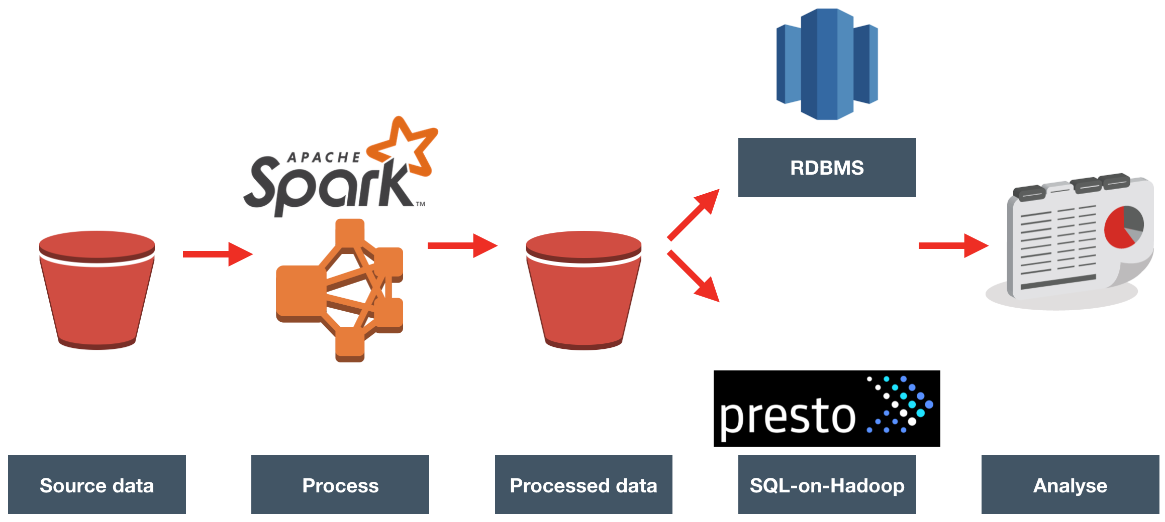
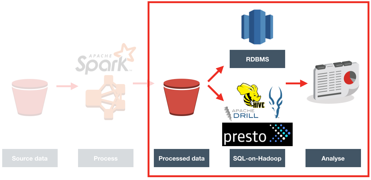
We recently did a project we did for a client, exploring the benefits of Spark-based ETL processing running on Amazon's Elastic Map Reduce (EMR) Hadoop platform. The proof of concept we ran was on a very simple requirement, taking inbound files from a third party, joining to them to some reference data, and then making the result available for analysis.

The background to the project is here, I showed here how I built up the prototype PySpark code on my local machine, and then here how it could be run on Amazon's EMR hadoop platform automatically.

In this article I'm going to discuss the options for analysing the data and producing reports from it.

Squeegee Your Third Eye

Where do we store data for analysis? Databases, right? That's what we've always done. Whether Oracle, SQL Server, or even Redshift - we INSERT, UPDATE, and SELECT our data in a database, and all is well and happy with the world.

But ... what if you didn't need a database per se to query your data?

One of the things I wanted to explore during this project was the feasibility and response times that "SQL on Hadoop" engines could bring. Hive is probably the most well known of these, with other options including Apache Impala (incubating), Apache Drill, Presto, and even Oracle's Big Data SQL. All these tools read data that is not stored in a proprietory database format but stored in an open format, such a simple text file, on open storage platform such as HDFS. More commonly, formats (also open, non-proprietory) which are optimised for performance such as Parquet or ORC are used.

The advantage of these is that they provide multiple options for working with your data, starting from the same base storage place (usually HDFS, or S3). If one tool has benefits over another in a particular processing or analytics scenario we have the option to switch, without having to do anything to the actual data at rest itself. Contrast this to the implicit assumption that the data starts in an RDBMS (such as Oracle). With the data in a proprietary database the only options for switching tools are which ones you use to submit workload (over JDBC/ODBC/OCI etc). If another database platform is better in a given use case you end up either duplicating the data, or re-platforming the data entirely.

So whilst the flexibility of SQL-on-Hadoop is very appealing, there are limitations to it currently, in areas including performance and levels of ANSI SQL support.

Throughout this evaluation, my considerations were:

  • Performance. The client we were doing this project for performs both batch querying as well as ad-hoc analytics
  • Complexity, in two areas:
    • Configuration and optimisation : The more configuration and careful tending that a platform needs, the greater the overall cost. Oracle may have its license implications compared to open-source software, but how to operate it for optimal performance is well known and documented. It's also an extremely mature product, having solved many of the problems that newer technologies are only just starting to realise, let alone solve.
    • Load process: Whilst the SQL-on-Hadoop engines don't "load" the data, they sometimes require it to be laid out in a particular pattern of folders, or in a particular format for optimal performance.
  • Compatibility. JDBC or ODBC interfaces are needed to be able to use the tool with BI tools such as OBIEE or Oracle's Data Visualization Desktop. As well as the interface, the SQL language support needs to be sufficient for analytical queries.

For an overview of SQL-on-Hadoop engines see this presentation from Greg Rahn. It's a couple of years old but pretty much still current bar the odd version and feature change.

Redshift

Redshift is not SQL-on-hadoop - it is a full-blown database. Specifically, it is a proprietory implementation of Postgres by Amazon, running as a service on their cloud. Just as you can provision an EMR cluster of any required size, you can do the same for Redshift. As your capacity and processing requirements change, you can scale your Redshift cluster up and down.

Redshift has both JDBC and ODBC drivers, making it accessible from both Data Visualization Desktop (supported) and OBIEE (works, but not supported).

To work with Redshift you can use a tool just as SQL WorkbenchJ, or the psql commandline tool. I installed the latter on my Mac using brew and brew install postgres.

With the processed data held on S3, loading it into Redshift is as simple as defining the table (with standard CREATE TABLE DDL), and then issuing a COPY command:

COPY ACME FROM 's3://foobar-bucket/acme_enriched/'
CREDENTIALS 'aws_access_key_id=XXXXXXXXXXXXXX;aws_secret_access_key=YYYYYYYYYYYY'
CSV
NULL AS 'null'
MAXERROR 100000
;

This takes any file under the given S3 path (and subfolders), parses it as a CSV, and loads it into the table. It presumes that the columns in the table are in the order that they are in the CSV file.

As a rough idea of load timings across several separate load jobs:

  • 2M rows in 10 minutes
  • 6M rows in 30 minutes
  • 23M rows in 1h18 minutes

Just like with the Spark coding, I didn't undertake any performance optimisations or 'good practices'. No sort keys or distribution configuration - just however it came by default, I used.

Out of the box, response times were pretty good - here's a sample of the queries. They're going across the same set of data (23M rows), stored on Redshift with no defined sort keys, distribution keys, etc - just however it comes out of the box with a vanilla CREATE TABLE DDL.

  • COUNT all records - 0.2 seconds

      dev=# select count(*) from acme3;
      count
      ----------
      23011785
      (1 row)
    
      Time: 225.053 ms
    
  • COUNT, GROUP BY - 2.0 seconds

      dev=# select country,site_category, count(*) from acme3 group by country,site_category;
      country | site_category  |  count
      ---------+----------------+---------
      GB      | Indirect       |  512519
      [...]
      (34 rows)
    
      Time: 2043.805 ms
    
  • COUNT, GROUP BY day (with DATE_TRUNC function) - 1.6 seconds

      dev=# select date_trunc('day',date_launched),country,count(*) from acme3 group by date_trunc('day',date_launched),country;
      date_trunc           | country | count
      ---------------------+---------+--------
      2016-01-01 00:00:00  | GB      |  24795
      [...]
      (412 rows)
    
      Time: 1625.590 ms
    
  • COUNT, GROUP BY week (with DATE_TRUNC function) - 3.8 seconds

      dev=# select date_trunc('week',date_launched),country,count(*) from acme3 group by date_trunc('week',date_launched),country;
      date_trunc           | country |  count
      ---------------------+---------+---------
      2016-01-18 00:00:00  | GB      | 1046417
      2016-01-25 00:00:00  | GB      |  945160
      2016-02-01 00:00:00  | GB      | 1204446
      2016-02-08 00:00:00  | GB      |  874694
      [...]
      (77 rows)
    
      Time: 3871.230 ms
    
  • COUNT, GROUP BY, WHERE, ORDER BY - 5.4 seconds

      dev=# select supplier, product, product_desc,count(*)  from acme3 where lower(product_desc) = 'beans' group by supplier,product,product_desc order by 4 desc limit 2;
      supplier             |      product    | product_desc | count
      ---------------------+-----------------+--------------+------
      ACME BEANS CO        | baked beans     | BEANS        |  2967
      BEANZ MEANZ          | beans + saus    | Beans        |  2347
      (2 rows)
    
      Time: 5427.035 ms
    

Hive (on Tez)

Hive enables you to run queries with SQL-like language (Hive QL) on data stored in various places including HDFS, and S3. It supports multiple formats of data, including simple delimited text files like CSV, and more advanced formats such as Parquet.

The version of Hive that I was using on EMR was automagically configured to use Tez as its execution engine, instead of the traditional map/reduce of the original Hadoop platform.

To query the data, simply define an EXTERNAL table. Why an EXTERNAL table? Well if you just define a TABLE, and then drop it ... it will also delete the underlying data. It's one of those syntax decisions that makes brutally logical sense, but burnt me and I'm sure has burnt many others. But, you won't do it again (or at least, not for a while).

CREATE EXTERNAL TABLE acme
(
product_desc STRING,
product STRING,
product_type STRING,
supplier STRING,
date_launched TIMESTAMP,
[...]
)
ROW FORMAT DELIMITED FIELDS TERMINATED BY ','
STORED AS TEXTFILE
LOCATION 's3://foobar-bucket/acme_enriched';

With the table defined you can test that it works using the LIMIT clause to only pull back some of the records:

hive> select product_desc,supplier,country from acme3 limit 5;
OK
Baked Beans       BEANZ MEANZ  GB
Tinned Tom      VEG CORP      GB
Tin Foil  FOIL SOLN   GB
Shreddies    CRUNCHYCRL     GB
Lemonade  FIZZ POP        GB

Whilst Hive technically enables you to query your data, the response times are so high that it's not even really a candidate for batch reporting.

Here's a couple of examples against a very small set of data, held in CSV format:

hive> select count(*) from acme;
21216
Time taken: 58.063 seconds, Fetched: 1 row(s)

hive> select country,count(*) from acme group by country;
US      21216
Time taken: 50.646 seconds, Fetched: 1 row(s)

Tez helpfully provides a progress report of queries, such as this one here - a simple count of all rows, on a much larger dataset (25M rows, CSV files). After seven minutes, I gave up - with 3% of the query complete

hive> select count(*) from acme3;
Query ID = hadoop_20161019112007_cca7d37f-c5af-47f2-9d7d-3187342fbbb3
Total jobs = 1
Launching Job 1 out of 1
Tez session was closed. Reopening...
Session re-established.


Status: Running (Executing on YARN cluster with App id application_1476873946157_0002)

----------------------------------------------------------------------------------------------
VERTICES      MODE        STATUS  TOTAL  COMPLETED  RUNNING  PENDING  FAILED  KILLED
----------------------------------------------------------------------------------------------
Map 1            container       RUNNING  107601       3740        5   103856       0       6
Reducer 2        container       RUNNING      1          0        1        0       0       0
----------------------------------------------------------------------------------------------
VERTICES: 00/02  [>>--------------------------] 3%    ELAPSED TIME: 442.36 s
----------------------------------------------------------------------------------------------

As with elsewhere in the exercise - I'm well aware that there are optimisations that could be made that could help with response time, such as storing the data in more optimal formats (ORC/Parquet) and layouts (partitioning) as well as compresing it.

Don't write Hive off though - the latest versions (being developed by Hortonworks, and not on EMR yet) are moving to use in-memory components and competing well against Impala.

Impala

Impala is Cloudera's open-source offering in the SQL-on-Hadoop space. I was hoping to try out Impala against the data in S3, especially given a recent post by Cloudera with some promising performance metrics. Unfortunately this was for Impala 2.6, and the only version available prebuilt on EMR was 1.2.4. Given time, it would have been possible to build my own CDH-based Hadoop cluster (using Director to automate it) with the latest version of Impala installed - but this will have to be for another day. The current Cloudera documentation also suggests that S3 is:

[...]more suitable for holding 'cold' data that is only queried occasionally

although it's not clear if that's still true in the context of the latest Impala S3 optimisations.

Presto

Presto is an open source project that originated at Facebook. Similar to Apache Drill (below), it can query across data (and federate the results) from multiple sources including Hive (and thus S3), MongoDB, MySQL, and even Kafka.

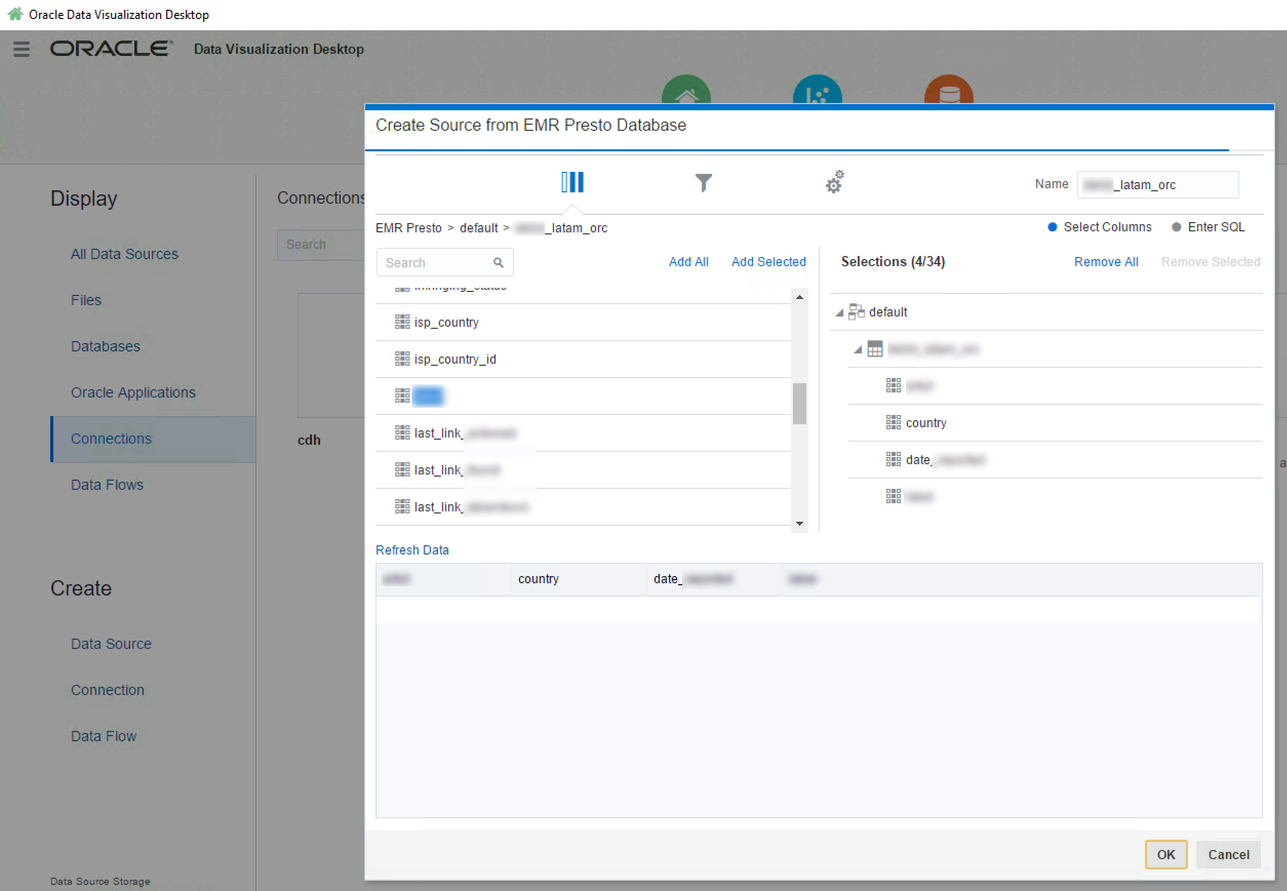
For Presto to query against the data in S3, you need to define the table in Hive first. Presto uses the Hive metastore to retrieve the definition of the table, and carries out the actual query execution itself. First, a simple smoke test that we can pull back some data:

$ presto-cli --catalog hive --schema default

presto:default> select product_desc,supplier,country from acme limit 5;
product_desc | supplier | country
-------+-------+---------
(0 rows)

Query 20161019_110919_00004_ev4hz, FINISHED, 1 node
Splits: 1 total, 1 done (100.00%)
0:01 [0 rows, 0B] [0 rows/s, 0B/s]

No data. Hmm. The exact same query against the same Hive table does return data. Turns out that Presto, by default, won't recursively query subfolders, whilst Hive, by default, does. After amending /etc/presto/conf.dist/catalog/hive.properties to set hive.recursive-directories=true and restarting Presto (sudo restart presto-server) on each EMR node, I then got data back:

presto:default> select count(*) from acme_latam;
_col0
---------
1993955
(1 row)

Query 20161019_200312_00003_xa352, FINISHED, 2 nodes
Splits: 44 total, 44 done (100.00%)
0:10 [1.99M rows, 642MB] [203K rows/s, 65.3MB/s]

This was against a 1.9M row dataset, held in CSV format. Run again soon after, and the response time was 3 seconds.

Querying a bigger set of data was slower - 4 minutes for 23M rows of data:

presto:default> select count(*) from acme3;
_col0
----------
23105948
(1 row)

Query 20161019_200815_00006_xa352, FINISHED, 2 nodes
Splits: 52,970 total, 52,970 done (100.00%)
4:04 [23.1M rows, 9.1GB] [94.8K rows/s, 38.2MB/s]

Same timing for doing a GROUP by on the data too:

presto:default> select country,site_category, count(*) from acme3 group by country,site_category;
country |  site_category     |  _col2
--------+--------------------+----------
GB      | Price comparison   |     146
GB      | DIRECT RETAIL      |   10903
[...]
Query 20161019_201443_00013_xa352, FINISHED, 2 nodes
Splits: 52,972 total, 52,972 done (100.00%)
4:54 [23.1M rows, 9.11GB] [78.6K rows/s, 31.7MB/s]

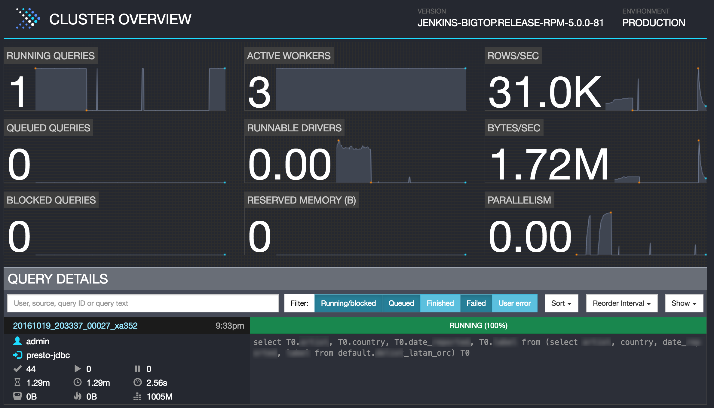
Presto includes a swanky web interface for seeing the status and execution of queries

Loading to ORC

Taking a brief detour into one of the most common recommendations for performance with Presto - storing data in ORC format.

First, in Hive, I created an ORC-stored table:

CREATE EXTERNAL TABLE acme_orc
(
product_desc STRING,
product STRING,
product_type STRING,
supplier STRING,
date_launched TIMESTAMP,
[...]
)
STORED AS ORC
LOCATION 's3://foobar-bucket/acme_orc/';

and then loaded a small sample of data:

hive> insert into acme_orc select * from acme_tst;

Querying it in Presto:

presto:default> select count(*) from acme_orc;
_col0
-------
29927
(1 row)

Query 20161019_113802_00008_ev4hz, FINISHED, 1 node
Splits: 2 total, 2 done (100.00%)
0:01 [29.9K rows, 1.71MB] [34.8K rows/s, 1.99MB/s]

With small volumes this was fine - 90 seconds to load 30k rows into an ORC-stored table, and a second to then query that from Presto with a count across all rows.

Loading 1.9M rows into an ORC-stored table took 30 minutes, and didn't actually (on the surface) speed things up. Caveat: this was a first pass at optimisation; there'll be a dozen settings and approaches to try out before any valid conclusions can be drawn from it:

  • COUNT GROUP BY from 1.9M rows, ORC - 3 seconds

      presto:default> select country,site_category, count(*) from acme_latam_orc group by country,site_category;
      country | site_category |  _col2
      ---------+---------------+---------
      LATAM   | null          | 1993955
      (1 row)
    
      Query 20161019_202206_00017_xa352, FINISHED, 2 nodes
      Splits: 46 total, 46 done (100.00%)
      0:03 [1.99M rows, 76.2MB] [790K rows/s, 30.2MB/s]
    
  • COUNT over 1.9M rows, CSV - 3 seconds

      presto:default> select country,site_category, count(*) from acme_latam group by country,site_category;
      country | site_category |  _col2
      ---------+---------------+---------
      LATAM   | null          | 1993955
      (1 row)
    
      Query 20161019_202241_00018_xa352, FINISHED, 2 nodes
      Splits: 46 total, 46 done (100.00%)
      0:03 [1.99M rows, 642MB] [575K rows/s, 185MB/s]
    
  • Function and filter, 1.9M rows, ORC

      presto:default> select count(*) from acme_latam_orc where lower(product_desc) = 'eminem';
      _col0
      -------
      2107
      (1 row)
    
      Query 20161019_202558_00019_xa352, FINISHED, 2 nodes
      Splits: 44 total, 44 done (100.00%)
      0:04 [1.99M rows, 76.2MB] [494K rows/s, 18.9MB/s]
    
  • Function and filter, 1.9M rows, CSV

      presto:default> select count(*) from acme_latam where lower(product_desc) = 'eminem';
      _col0
      -------
      2107
      (1 row)
    
      Query 20161019_202649_00020_xa352, FINISHED, 2 nodes
      Splits: 44 total, 44 done (100.00%)
      0:03 [1.99M rows, 642MB] [610K rows/s, 196MB/s]
    

Trying to load greater volumes (23M rows) to ORC was unsuccessful, due to memory issues with the Hive execution.

Status: Running (Executing on YARN cluster with App id application_1476905618527_0004)

----------------------------------------------------------------------------------------------
VERTICES      MODE        STATUS  TOTAL  COMPLETED  RUNNING  PENDING  FAILED  KILLED
----------------------------------------------------------------------------------------------

----------------------------------------------------------------------------------------------
VERTICES: 00/00  [>>--------------------------] 0%    ELAPSED TIME: 13956.69 s
----------------------------------------------------------------------------------------------
Status: Failed
Application application_1476905618527_0004 failed 2 times due to AM Container for appattempt_1476905618527_0004_000002 exited with  exitCode: 255

In the Tez execution log was the error

Diagnostics: Container [pid=4642,containerID=container_1476905618527_0004_01_000001] is running beyond physical memory limits. Current usage: 1.0 GB of 1 GB physical memory used; 2.7 GB of 5 GB virtual memory used. Killing container.

With appropriate investigation (and/or smaller chunks of data loading) this could obviously be overcome, but for now halted any further investigation into ORC's usefulness. The other major area to investigate would be partitioning of the data.

A final note on performance - this blog does a comparison of Presto querying data held in S3 vs HDFS on EMR. HDFS on EMR is quicker, generally about 1.5 times or so - but you of course need your data loaded into HDFS on a running EMR cluster, whereas S3 is there on demand whenever you want it.

Drill

Apache Drill is another open-source tool, similar in concept to Presto, in that it enables querying across data held in multiple sources. I've written about it previously here and here. Whilst EMR has an option to provision a Drill cluster as part of an EMR build, it didn't seem to work when I tried it - and with Presto running I didn't spend the time digging into Drill. Given another time and project though, I'd definitely be looking to run it against this kind of data to see how it handled it. A recent thread on the Drill mailing list gave some interesting information on performance.

Athena

Amazon's Athena tool was announced at re:Invent 2016. Even though it was made GA after the client project being discussed here and therefore not evaluated, it is definitely worth mentioning. It provides "serverless" SQL querying of data held in S3. Under the covers it uses Presto (which is one of the tools I evaluated above). The benefit of Athena is that you wouldn't need to provision and configure actual servers to use Presto. You work with it through the web-based interface, or JDBC. This is a pretty big point to make - you can query your data, held in an open format, on demand, using SQL, without having to move it into a database or build a server to run a query engine.

Athena looks interesting, but one of the main things that struck me about it was that it is not something you would simply point at piles of data on S3 and build your analytics systems on. The cost is per query, and is currently $5 per TB scanned. FIVE DOLLARS, per terabyte of data SCANNED. Not retrieved. Scanned. So in order to not run up big AWS bills if you've got lots of data, you're going to need to do smart things to reduce the size of data scanned. Partitioning your data, and compressing it, will both help. As it happens, these are the things that are going to increase performance too, so it's not wasted effort. There's a good writeup here demonstrating Athena, and the difference that using an appropriate storage format for the data makes to performance and volumes of data scanned (and thus cost).

The cost consideration is a crucial point, because it means that data 'engineering' is still needed in any system you plan to build Athena on top of as the query engine. Sure, you can use it for adhoc 'fishing' expeditions in your 'data lake' (sorry....). Here the benefit of sifting through vast and disparate data without having to transform and/or load it into a queryable form first will probably outweigh the ad-hoc costs (remember : $5 per TB scanned). But as I said, if you're engineering Athena into your system as the SQL engine of top of data at rest in S3, you'll want to invest in the necessary wrangling in order to store the data (a) partitioned and (b) compressed.

You can read more about Athena here.

Front End Tools

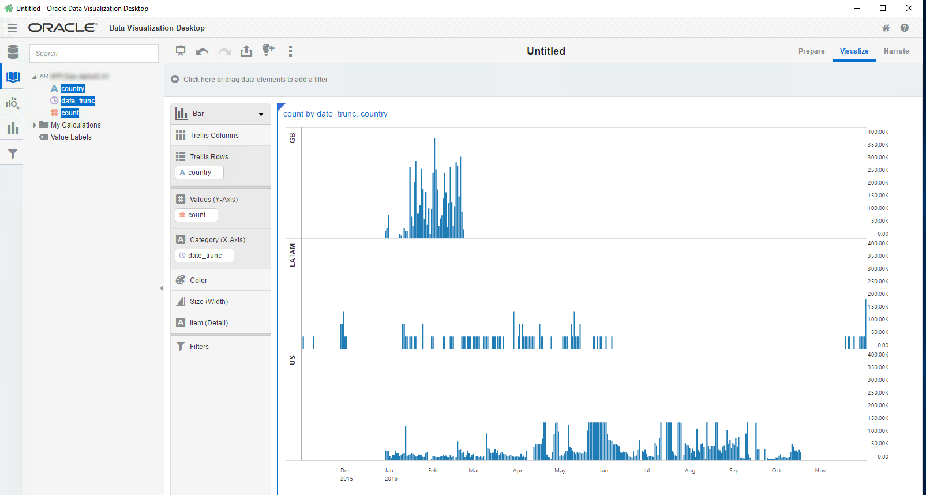
All of the exploration so far has been from the commandline, but users want their data visually. The client for whom we were doing this work currently use OBIEE and BI Publisher to deliver the data. Both Redshift and Presto have JDBC and ODBC drivers, which means that they should work with OBIEE (although neither are on the supported databases list). Oracle's Data Visualization Desktop tool is also of interest here, bringing with it native support for both Redshift and Presto (beta).

A tool that we didn't examine, but is directly relevant given the Amazon context, is Quicksight. Currently in closed-preview Released in mid-November 2017, this is a cloud-based tool that enables querying of data in many sources including Redshift -- but also S3 itself.

Summary

For interactive analysis, Redshift performed well straight off. However, with some of the in-memory capabilities of the SQL-on-Hadoop engines, and the appeal of simply provisioning compute to query data held on S3 when required, it would be interesting to spend some time digging into the recommended optimisations and design patterns to see just how fast the querying could be.

Since all the query engines considered support JDBC, and any respectable front-end tool can query JDBC, we're not constrained in the choice of one by the other. Hooray for open standards enabling optimal choice and pairing of technologies! I liked using Oracle DV Desktop as it's a simple install and quick to get visualisations out of. Ultimately the choice of tool would come down to factors including complexity of requirements, scale of deployment - and of course, cost.

In the final article in this series we'll take a recap over the whole project, and look at some of the broader points of interest to draw from it.


ETL Offload with Spark and Amazon EMR - Part 5 - Summary

$
0
0

This is the final article in a series documenting an exercise that we undertook for a client recently. Currently running an Oracle-based datawarehouse platform, the client asked for our help in understanding what a future ETL and reporting platform could look like, given the current landscape of tools available. You can read the background to the project, how we developed prototype code, deployed it to Amazon, and evaluated tools for analysing the data.

Whilst the client were generally aware of new technologies, they wanted a clear understanding of what these looked like in practice. Is it viable, as is being touted, to offload ETL entirely to open-source tools? Could they do this, without increasing their licensing costs?

The client are already well adopted to newer technologies, running their entire infrastructure on the Amazon Web Services (AWS) cloud. Given this usage of AWS, our investigation was based around deployment of the Elastic Map Reduce (EMR) Hadoop platform. Many of the findings made during the investigation are as applicable to other Hadoop platforms though, including CDH running on Oracle's Big Data Appliance.

We isolated a single process within the broader part of the client's processing estate for exploration. The point of our study was not less to implement this specific piece of functionality in the most optimal way, but to understand how in general processing would look on another platform in an end-to-end flow. Before any kind of deployment into Production of this design there would be further iterations, particularly around performance. These are discussed further below.

Overview of the Solution

The source data landed in Amazon S3 (similar in concept to HDFS), in CSV format, once per hour. We loaded each file, processed it to enrich it with reference data, and wrote it back to S3.

The enriched data was queried directly, with Presto, and also loaded into Redshift for querying there.

Oracle's Data Visualization Desktop was used as the front end for querying.

Benefits

Cost Benefits

  • By moving ETL processing to Hadoop-based platform, we free up capacity (and potentially licensing costs) on the existing commerical RDBMS (Oracle) where the processing currently takes place
  • Costs are further reduced by the 'elastic' provisioning and cost model of the cloud service. You only pay for the size of the cluster necessary for your workload, for the duration that it took to execute.

Technology Benefits

In this solution we have taken advantage of the decoupling of storage from compute. This is a significant advantage that cloud technology brings.

  • Amazon S3 provides the durable data store for our data (whether CSV, Parquet, or any other data format). With S3 you simply pay for the storage that you use. S3 can be accessed by dozens of client libraries as well as HDFS-compatible APIs. Data in S3 is completely compute-target agnostic. Contrast this to data sat in your proprietory RDBMS database, and if you want to process or analyse this in another system.
  • In this instance we wanted to enrich the data, and proved Spark as an appropriate tool to do so. Running on Elastic Map Reduce we could provision this automagically, run our processing, and have the EMR cluster terminate itself once complete. The compute part of the equation is entirely isolated, and can be switched in and our of the architecture as required.

Moving existing workloads to the cloud is not just a case of provisioning servers running in someone else's data centre to perform the same work as before. To truly benefit (dare I say, leverage) from the new possibilities, it makes sense to re-architect how you store your data and perform processing on it.

As well as the benefit of cloud technology, we can see that we don't even need an RDBMS for much of this enrichment and transformation work. Redshift has proved to be useful for interactive analysis of the data, but the processing of the data that would typically get done within an RDBMS (with associated license costs) can instead be done on technology such as Spark.

Broader Observations

The world of data and analytics is changing, and there are some interesting points that this project raised, which I discuss below.

Cloud

The client for whom we carried out this work are already cloud 'converts', running their entire operation on AWS already. They're not alone in recognising the benefits of Cloud, and it's going to be interesting to see the rate at which adoption continues to occur elsewhere, particularly in the Oracle market as they ramp up their offerings.

Cloud Overview

The Cloud is of course a big deal nowadays, whether in the breathless excitement of marketing talk, or the more gradual realisation amongst more technical folk that The Cloud brings some serious benefits. There are three broad flavours of Cloud - Infrastructure, Platform, and Software (IaaS, PaaS, SaaS respectively):

  • At the lowest level, you basically rent access to tin (hardware). Infrastructure-as-a-service (IaaS) can include simply running virtual machines on someone else's hardware, but it's more clever than that. You get the ability to provision storage separately from compute, and all with virtualised networking too. Thus you store your data, but don't pay for the processing until you want to. This is a very long way from working out how big a server to order for installation in your data centre (or indeed, a VM to provision in the cloud) - how many CPUs, how much RAM, how big the hard disks should be - and worrying about under- or over-provisioning it.

    With IaaS the components can be decoupled, and scaled elastically as required. You pay for what you use.

    The additional benefit of IaaS is that someone else manages the actual hardware; machine outages, disk failures, and so on, are all someone else's concern.

  • IaaS can sometimes still be a lot of work; after all, you still have the manage the servers, or architect and manage the decoupled components such as storage and compute. The next 'aaS' up in Platform as a Service (PaaS). Here, the "platform" is provided and managed for you.

    A clear example of PaaS is the Hadoop platform. You can run a Hadoop cluster yourself, whether on Oracle's Big Data Appliance (BDA), or maybe on your own hardware (or indeed, on IaaS in the cloud) but with a distribution such as Cloudera's CDH. Point being, you still have to manage it, to tune your Hadoop parameters, and so on. Hadoop as a platform in the cloud (i.e. PaaS) is offered by many companies, including the big vendors, such as Oracle (Big Data Cloud Service), Microsoft (HDInsight), Google (Dataproc) -- and then the daddy of them all, Amazon with it's Elastic Map Reduce (EMR) platform

    Another example of PaaS is Oracle's BI Cloud Service (BICS), in which you build and run your own RPD and reports, but Oracle look after the actual server processes.

  • Software as a Service (SaaS) is where everything is provisioned and managed for you. Whereas on PaaS you still write the code that's to be run (whether a Spark routine on Hadoop, or BI metadata model on BICS), on SaaS someone has already done that too. You just provide the inputs, which obviously depend on the purpose of the SaaS. Something like GMail is a good example of SaaS. You're not having to write the web-based email, you're not having to provision the servers on which to run that - you simply utilise the software.

Cloud's Benefit to Analytics

Cloud brings benefits - but also greater subtleties to our solutions. Instead of simply provisioning one or more servers on which to hold our data and process it, we start to unpick this into separate components. In the context of this study, we have:

  • Data at rest, on S3. This is storage paid for simply based on how much you use. Importantly, you don't have to have a server (or in more abstract terms, 'compute') running. It's roughly analogous to network mounted storage. You can access S3 externally to AWS, such as your laptop or a server in your data centre. You can also access it, obviously, from within the AWS ecosystem. You can even use S3 to serve up files just as a web server would.
  • Compute, on EMR. How often do you need to carry out transformations and processing on your data? Not continuously? Then why pay for a server to sit idle the rest of the time? What about the size of the server that it does run on - how many CPUs do you need? How many nodes in your cluster? EMR solves both these problems, by enabling you to provision a Hadoop cluster of any size and spec, on demand - and optionally, terminate itself once it's completed its work so that you only pay for the compute time necessary.
  • Having a bunch of data sat around isn't going to bring any value to the business, without Analytics and a way of presenting that to the user. This could be done either through loading the data into a traditional RDBMS such as Oracle, or Redshift, and analysing it there - or potentially through one of the new generation of "SQL on Hadoop" engines, such as Impala or Presto. There's also Athena which is a SQL interface directly to data in S3 - you don't even need to be running a Hadoop cluster to use this.

Innovation vs Execution (or, just because you can, doesn't mean you should)

The code written during this exercise could, with a bit of tidying up, be run in Production. As in, it does the job that it was built to do. We could even expand it to audit row counts in and out, report duff data, send notifications when complete. What about the next processing requirement that comes in? More bespoke code? And more? At some point we'd probably end up refactoring a whole bunch of it into some kind of framework. Into that framework we'd obviously want good things like handling SCDs, data lineage, and more. Welcome to re-inventing the in-house ETL wheel. Whether Spark jobs nowadays, PL/SQL ten years ago, or COBOL routines a decade before that - doing data processing at a wider scale soon becomes a challenge. Even with the best coders (or 'engineers' as they're now called) in the world, you're going to end up with a bespoke platform that's relient on inhouse skills to support and maintain. That presumes of course that you can find the relevant skills in the market to write all the processing and transformations that you need - and support them, of course. As you aquire new staff, they'll need to be trained on your code base - and suddenly the "free" technology platform isn't appearing so cheap.

Before you shoot me down for a hyperbolic strawman argument, there is an important dichotomy to draw here, between innovation and execution. Applicable to the world of big data in general, it is a useful concept spelt out in the Oracle Information Management & Big Data Reference Architecture. For data to provide value, it doesn't have to land straight away into the world of formalised development processes, Production environments, and so on. A lot of the time you will want to 'poke around' with it, to explore it -- to innovate. Of the technology base out there, you may not know which tool, or library, is going to yield the best results. This is where the "discovery lab" comes in, and where the type of hand-cranked Spark coding that I've demonstrated sits:

Sometimes, work done in innovation is complete once it's done. As in, it has answered the required business question, and provided its value. But a lot of the time though it will simply establish and prove the process that is to be applied to the data, that then needs taking through to the execution layer. This is often called, in an abuse of the English language, "productionisation" or "industrialisation". This is where the questions of code maintenance and scalability need to be seriously considered. And this is where you need a scalable and maintainable approach to the design, management, and orchestration of your data processing - which is exactly what a tool like Oracle Data Integrator (ODI) provides.

ODI is the premier DI tool on the market, with good support for "big data" technologies, including the ability to generate Spark code to perform transformation. It can be deployed to run on Amazon's EMR, as illustrated here, as well as Oracle's Cloud platform. As can be seen from this presentation from Oracle Open World in September 2016, there's additional capabilities coming including around Kafka, Spark Streaming, and Cassandra.

Another route to examine, alongside ODI, is the ecosystem within AWS itself around code execution and orchestration with tools such as Lambda, Data Pipeline, and Simple Workflow Service. There's also AWS Glue, which like Athena was announced at re:Invent 2016. This promises three key things of crucial importance here:

  • A Data Catalog, populated automatically, and not only just supporting multiple formats and sources, but including automatic classification (e.g. "Web Log") of the data itself.
  • Automatic generation of ETL code. From the release announcement notes this looks like it is pySpark-based code. So the code that I put together for this exercise here, manually (and at times, painfully), could be automagically generated based on source/target and operators required. The announcement notes also specifically mention the inclusion of standard ETL processes such as handling bad data
  • Orchestration and management of ETL jobs. One of my main objections above to taking 'proof of concept' pySpark code and trying to use it in a Production scenario is that you end up with a spaghetti of scripts, which are a nightmare to maintain and support. If Glue lives up to its promises, we'd pretty much get the best of all worlds - a flexible yet robust platform.

Hadoop Ecosystems

A single vendor for your IT platform gives you "one throat to choke" when it comes to support, which is usually a good thing. But if that vendor's platform is closed and proprietary it makes leaving it, or even just making use of alternative tools with it, difficult. One of the evangelical claims made about the new world of open source software is that the proliferation of open standards would spell an end to vendor lockin. I was interested to see during the course of this exercise a few examples where the big vendors subtly pushed you towards their own tool of choice, or away from an alternative.

For example, Amazon EMR makes available Presto as part of the default build, but to run the latest version of Impala you'd have to install it yourself. Whilst it is possible to install it yourself, of course, this added friction makes it less likely that people will. This friction increases when we consider that the software usually needs installing - and configuring - across multiple the nodes of the Hadoop cluster. Given an open field of tools all purporting to do the same or similar things, any impedance to using one over the other will count. The same argument could be made for the CDH distribution, in which Impala is front and center, and deploying Presto or Drill would be a manual exercise. Again, yes, installing it may be relatively trivial - but manual download and deployment across a cluster is never going to win out over a one-click deploying from a centralised management console.

This is a long way from any kind of vendor lockin, but it is worth bearing in mind that walls, albeit thin ones, are being built around these various gardens in the Hadoop ecosystem.

Summary

I hope you've found this series of article useful. You can find a list of them below. In the meantime, please do get in touch if you'd like to find out more about how Rittman Mead can help you on your data and analytics journey!


You can listen to a discussion of this project, along with other topics including OBIEE, in an episode of the Drill to Detail podcast here.

Getting Started with Spark Streaming, Python, and Kafka

$
0
0

Last month I wrote a series of articles in which I looked at the use of Spark for performing data transformation and manipulation. This was in the context of replatforming an existing Oracle-based ETL and datawarehouse solution onto cheaper and more elastic alternatives. The processing that I wrote was very much batch-focussed; read a set of files from block storage ('disk'), process and enrich the data, and write it back to block storage.

In this article I am going to look at Spark Streaming. This is one of several libraries that the Spark platform provides (others include Spark SQL, Spark MLlib, and Spark GraphX). Spark Streaming provides a way of processing "unbounded" data - commonly referred to as "streaming" data. It does this by breaking it up into microbatches, and supporting windowing capabilities for processing across multiple batches. You can read more in the excellent Streaming Programming Guide.

(image src)

Why Stream Processing?

Processing unbounded data sets, or "stream processing", is a new way of looking at what has always been done as batch in the past. Whilst intra-day ETL and frequent batch executions have brought latencies down, they are still independent executions with optional bespoke code in place to handle intra-batch accumulations. With a platform such as Spark Streaming we have a framework that natively supports processing both within-batch and across-batch (windowing).

By taking a stream processing approach we can benefit in several ways. The most obvious is reducing latency between an event occurring and taking an action driven by it, whether automatic or via analytics presented to a human. Other benefits include a more smoothed out resource consumption profile. We can avoid the very 'spiky' demands on CPU/memory/etc every time a batch runs by instead processing the same volume of data processed but in smaller intervals. Finally, given that most data we process is actually unbounded ("life doesn't happen in batches"), designing new systems to be batch driven - with streaming seen as an exception - is actually an anachronism with roots in technology limitations that are rapidly becoming moot. Stream processing doesn't have to imply, or require, "fast data" or "big data". It can just mean processing data continually as it arrives, and not artificially splitting it into batches.

For more details and discussion of streaming in depth and some of its challenges, I would recommend:

Use-Case and Development Environment

So with that case made above for stream processing, I'm actually going to go back to a very modest example. The use-case I'm going to put together is - almost inevitably for a generic unbounded data example - using Twitter, read from an Apache Kafka topic. We'll start simply, counting the number of tweets per user within each batch and doing some very simple string manipulations. After that we'll see how to do the same but over a period of time (windowing). In the next blog we'll extend this further into a more useful example, still based on Twitter but demonstrating how to satisfy some real-world requirements in the processing.

I developed all of this code using Jupyter Notebooks. I've written before about how awesome notebooks are (along with Jupyter, there's Apache Zeppelin). As well as providing a superb development environment in which both the code and the generated results can be seen, Jupyter gives the option to download a Notebook to Markdown. This blog runs on Ghost, which uses Markdown as its native syntax for composing posts - so in fact what you're reading here comes directly from the notebook in which I developed the code. Pretty cool.

If you want can view the notebook online here, and from there download it and run it live on your own Jupyter instance.

I used the docker image all-spark-notebook to provide both Jupyter and the Spark runtime environment. By using Docker I don't have to really worry about provisioning the platform on which I want to develop the code - I can just dive straight in and start coding. As and when I'm ready to deploy the code to a 'real' execution environment (for example EMR), then I can start to worry about that. The only external aspect was an Apache Kafka cluster that I had already, with tweets from the live Twitter feed on an Apache Kafka topic imaginatively called twitter.

To run the code in Jupyter, you can put the cursor in each cell and press Shift-Enter to run it each cell at a time -- or you can use menu option Kernel -> Restart & Run All. When a cell is executing you'll see a [*] next to it, and once the execution is complete this changes to [y] where y is execution step number. Any output from that step will be shown immediately below it.

To run the code standalone, you would download the .py from Jupyter, and execute it from the commandline using:

/usr/local/spark-2.0.2-bin-hadoop2.7/bin/spark-submit --packages org.apache.spark:spark-streaming-kafka-0-8_2.11:2.0.2 spark_code.py

Preparing the Environment

We need to make sure that the packages we're going to use are available to Spark. Instead of downloading jar files and worrying about paths, we can instead use the --packages option and specify the group/artifact/version based on what's available on Maven and Spark will handle the downloading. We specify PYSPARK_SUBMIT_ARGS for this to get passed correctly when executing from within Jupyter.

import os
os.environ['PYSPARK_SUBMIT_ARGS'] = '--packages org.apache.spark:spark-streaming-kafka-0-8_2.11:2.0.2 pyspark-shell'

Import dependencies

We need to import the necessary pySpark modules for Spark, Spark Streaming, and Spark Streaming with Kafka. We also need the python json module for parsing the inbound twitter data

#    Spark
from pyspark import SparkContext
#    Spark Streaming
from pyspark.streaming import StreamingContext
#    Kafka
from pyspark.streaming.kafka import KafkaUtils
#    json parsing
import json

Create Spark context

The Spark context is the primary object under which everything else is called. The setLogLevel call is optional, but saves a lot of noise on stdout that otherwise can swamp the actual outputs from the job.

sc = SparkContext(appName="PythonSparkStreamingKafka_RM_01")
sc.setLogLevel("WARN")

Create Streaming Context

We pass the Spark context (from above) along with the batch duration which here is set to 60 seconds.

See the API reference and programming guide for more details.

ssc = StreamingContext(sc, 60)

Connect to Kafka

Using the native Spark Streaming Kafka capabilities, we use the streaming context from above to connect to our Kafka cluster. The topic connected to is twitter, from consumer group spark-streaming. The latter is an arbitrary name that can be changed as required.

For more information see the documentation.

kafkaStream = KafkaUtils.createStream(ssc, 'cdh57-01-node-01.moffatt.me:2181', 'spark-streaming', {'twitter':1})

Message Processing

Parse the inbound message as json

The inbound stream is a DStream, which supports various built-in transformations such as map which is used here to parse the inbound messages from their native JSON format.

Note that this will fail horribly if the inbound message isn't valid JSON.

parsed = kafkaStream.map(lambda v: json.loads(v[1]))

Count number of tweets in the batch

The DStream object provides native functions to count the number of messages in the batch, and to print them to the output:

We use the map function to add in some text explaining the value printed.

Note that nothing gets written to output from the Spark Streaming context and descendent objects until the Spark Streaming Context is started, which happens later in the code. Also note that pprint by default only prints the first 10 values.

parsed.count().map(lambda x:'Tweets in this batch: %s' % x).pprint()

If you jump ahead and try to use Windowing at this point, for example to count the number of tweets in the last hour using the countByWindow function, it'll fail. This is because we've not set up the streaming context with a checkpoint directory yet. You'll get the error: java.lang.IllegalArgumentException: requirement failed: The checkpoint directory has not been set. Please set it by StreamingContext.checkpoint().. See later on in the blog for details about how to do this.

Extract Author name from each tweet

Tweets come through in a JSON structure, of which you can see an example here. We're going to analyse tweets by author, which is accessible in the JSON structure at user.screen_name.

The lambda anonymous function is used to apply the map to each RDD within the DStream. The result is a DStream holding just the author's screenname for each tweet in the original DStream.

authors_dstream = parsed.map(lambda tweet: tweet['user']['screen_name'])

Count the number of tweets per author

With our authors DStream, we can now count them using the countByValue function. This is conceptually the same as this quasi-SQL statement:

SELECT   AUTHOR, COUNT(*)
FROM     DSTREAM
GROUP BY AUTHOR

Using countByValue is a more legible way of doing the same thing that you'll see done in tutorials elsewhere with a map / reduceBy.

author_counts = authors_dstream.countByValue()
author_counts.pprint()

Sort the author count

If you try and use the sortBy function directly against the DStream you get an error:

'TransformedDStream' object has no attribute 'sortBy'

This is because sort is not a built-in DStream function. Instad we use the transform function to access sortBy from pySpark.

To use sortBy you specify a lambda function to define the sort order. Here we're going to do it based on the number of tweets (index 1 of the RDD) per author. You'll note this index references being used in the sortBy lambda function x[1], negated to reverse the sort order.

Here I'm using \ as line continuation characters to make the code more legible.

author_counts_sorted_dstream = author_counts.transform(\
  (lambda foo:foo\
   .sortBy(lambda x:( -x[1]))))
author_counts_sorted_dstream.pprint()

Get top 5 authors by tweet count

To display just the top five authors, based on number of tweets in the batch period, we'll using the take function. My first attempt at this failed with:

AttributeError: 'list' object has no attribute '_jrdd'

Per my woes on StackOverflow a parallelize is necessary to return the values into a DStream form.

top_five_authors = author_counts_sorted_dstream.transform\
  (lambda rdd:sc.parallelize(rdd.take(5)))
top_five_authors.pprint()

Get authors with more than one tweet, or whose username starts with 'rm'

Let's get a bit more fancy now - filtering the resulting list of authors to only show the ones who have tweeted more than once in our batch window, or -arbitrarily- whose screenname begins with rm...

filtered_authors = author_counts.filter(lambda x:\
                                                x[1]>1 \
                                                or \
                                                x[0].lower().startswith('rm'))

We'll print this list of authors matching the criteria, sorted by the number of tweets. Note how the sort is being done inline to the calling of the pprint function. Assigning variables and then pprinting them as I've done above is only done for clarity. It also makes sense if you're going to subsequently reuse the derived stream variable (such as with the author_counts in this code).

filtered_authors.transform\
  (lambda rdd:rdd\
  .sortBy(lambda x:-x[1]))\
  .pprint()

List the most common words in the tweets

Every example has to have a version of wordcount, right? Here's an all-in-one with line continuations to make it clearer what's going on. Note that whilst it makes for tidier code, it also makes it harder to debug...

parsed.\
    flatMap(lambda tweet:tweet['text'].split(" "))\
    .countByValue()\
    .transform\
      (lambda rdd:rdd.sortBy(lambda x:-x[1]))\
    .pprint()

Start the streaming context

Having defined the streaming context, now we're ready to actually start it! When you run this cell, the program will start, and you'll see the result of all the pprint functions above appear in the output to this cell below. If you're running it outside of Jupyter (via spark-submit) then you'll see the output on stdout.

ssc.start()
ssc.awaitTermination()
-------------------------------------------
Time: 2017-01-11 15:34:00
-------------------------------------------
Tweets in this batch: 188

-------------------------------------------
Time: 2017-01-11 15:34:00
-------------------------------------------
(u'jenniekmz', 1)
(u'SpamNewton', 1)
(u'ShawtieMac', 1)
(u'niggajorge_2', 1)
(u'agathatochetti', 1)
(u'Tommyguns_____', 1)
(u'zwonderwomanzzz', 1)
(u'Blesschubstin', 1)
(u'Prikes5', 1)
(u'MayaParms', 1)
...

-------------------------------------------
Time: 2017-01-11 15:34:00
-------------------------------------------
(u'RitaBezerra12', 3)
(u'xKYLN', 2)
(u'yourmydw', 2)
(u'wintersheat', 2)
(u'biebercuzou', 2)
(u'pchrin_', 2)
(u'uslaybieber', 2)
(u'rowblanchsrd', 2)
(u'__Creammy__', 2)
(u'jenniekmz', 1)
...

-------------------------------------------
Time: 2017-01-11 15:34:00
-------------------------------------------
(u'RitaBezerra12', 3)
(u'xKYLN', 2)
(u'yourmydw', 2)
(u'wintersheat', 2)
(u'biebercuzou', 2)

-------------------------------------------
Time: 2017-01-11 15:34:00
-------------------------------------------
(u'RitaBezerra12', 3)
(u'xKYLN', 2)
(u'yourmydw', 2)
(u'wintersheat', 2)
(u'biebercuzou', 2)
(u'pchrin_', 2)
(u'uslaybieber', 2)
(u'rowblanchsrd', 2)
(u'__Creammy__', 2)

-------------------------------------------
Time: 2017-01-11 15:34:00
-------------------------------------------
(u'RT', 135)
(u'Justin', 61)
(u'Bieber', 59)
(u'on', 41)
(u'a', 32)
(u'&', 32)
(u'Ros\xe9', 31)
(u'Drake', 31)
(u'the', 29)
(u'Love', 28)
...
[...]

You can see the full output from the job in the notebook here.

So there we have it, a very simple Spark Streaming application doing some basic processing against an inbound data stream from Kafka.

Windowed Stream Processing

Now let's have a look at how we can do windowed processing. This is where data is processed based on a 'window' which is a multiple of the batch duration that we worked with above. So instead of counting how many tweets there are every batch (say, 5 seconds), we could instead count how many there are per minute. Here, a minutes (60 seconds) is the window interval. We can perform this count potentially every time the batch runs; how frequently we do the count is known as the slide interval.


Image credit, and more details about window processing, here.

The first thing to do to enable windowed processing in Spark Streaming is to launch the Streaming Context with a checkpoint directory configured. This is used to store information between batches if necessary, and also to recover from failures. You need to rework your code into the pattern shown here. All the code to be executed by the streaming context goes in a function - which makes it less easy to present in a step-by-step form in a notebook as I have above.

Reset the Environment

If you're running this code in the same session as above, first go to the Jupyter Kernel menu and select Restart.

Prepare the environment

These are the same steps as above.

import os
os.environ['PYSPARK_SUBMIT_ARGS'] = '--packages org.apache.spark:spark-streaming-kafka-0-8_2.11:2.0.2 pyspark-shell'
from pyspark import SparkContext
from pyspark.streaming import StreamingContext
from pyspark.streaming.kafka import KafkaUtils
import json

Define the stream processing code

def createContext():
    sc = SparkContext(appName="PythonSparkStreamingKafka_RM_02")
    sc.setLogLevel("WARN")
    ssc = StreamingContext(sc, 5)
    
    # Define Kafka Consumer
    kafkaStream = KafkaUtils.createStream(ssc, 'cdh57-01-node-01.moffatt.me:2181', 'spark-streaming2', {'twitter':1})
    
    ## --- Processing
    # Extract tweets
    parsed = kafkaStream.map(lambda v: json.loads(v[1]))
    
    # Count number of tweets in the batch
    count_this_batch = kafkaStream.count().map(lambda x:('Tweets this batch: %s' % x))
    
    # Count by windowed time period
    count_windowed = kafkaStream.countByWindow(60,5).map(lambda x:('Tweets total (One minute rolling count): %s' % x))

    # Get authors
    authors_dstream = parsed.map(lambda tweet: tweet['user']['screen_name'])
    
    # Count each value and number of occurences 
    count_values_this_batch = authors_dstream.countByValue()\
                                .transform(lambda rdd:rdd\
                                  .sortBy(lambda x:-x[1]))\
                              .map(lambda x:"Author counts this batch:\tValue %s\tCount %s" % (x[0],x[1]))

    # Count each value and number of occurences in the batch windowed
    count_values_windowed = authors_dstream.countByValueAndWindow(60,5)\
                                .transform(lambda rdd:rdd\
                                  .sortBy(lambda x:-x[1]))\
                            .map(lambda x:"Author counts (One minute rolling):\tValue %s\tCount %s" % (x[0],x[1]))

    # Write total tweet counts to stdout
    # Done with a union here instead of two separate pprint statements just to make it cleaner to display
    count_this_batch.union(count_windowed).pprint()

    # Write tweet author counts to stdout
    count_values_this_batch.pprint(5)
    count_values_windowed.pprint(5)
    
    return ssc

Launch the stream processing

This uses local disk to store the checkpoint data. In a Production deployment this would be on resilient storage such as HDFS.

Note that, by design, if you restart this code using the same checkpoint folder, it will execute the previous code - so if you need to amend the code being executed, specify a different checkpoint folder.

ssc = StreamingContext.getOrCreate('/tmp/checkpoint_v01',lambda: createContext())
ssc.start()
ssc.awaitTermination()
-------------------------------------------
Time: 2017-01-11 17:08:55
-------------------------------------------
Tweets this batch: 782
Tweets total (One minute rolling count): 782

-------------------------------------------
Time: 2017-01-11 17:08:55
-------------------------------------------
Author counts this batch:	Value AnnaSabryan	Count 8
Author counts this batch:	Value KHALILSAFADO	Count 7
Author counts this batch:	Value socialvidpress	Count 6
Author counts this batch:	Value SabSad_	Count 5
Author counts this batch:	Value CooleeBravo	Count 5
...

-------------------------------------------
Time: 2017-01-11 17:08:55
-------------------------------------------
Author counts (One minute rolling):	Value AnnaSabryan	Count 8
Author counts (One minute rolling):	Value KHALILSAFADO	Count 7
Author counts (One minute rolling):	Value socialvidpress	Count 6
Author counts (One minute rolling):	Value SabSad_	Count 5
Author counts (One minute rolling):	Value CooleeBravo	Count 5
...

[...]

-------------------------------------------
Time: 2017-01-11 17:10:10
-------------------------------------------
Tweets this batch: 5
Tweets total (One minute rolling count): 245

-------------------------------------------
Time: 2017-01-11 17:10:10
-------------------------------------------
Author counts this batch:	Value NowOnFR	Count 1
Author counts this batch:	Value IKeepIt2000	Count 1
Author counts this batch:	Value PCH_Intl	Count 1
Author counts this batch:	Value ___GlBBS	Count 1
Author counts this batch:	Value lauracoutinho24	Count 1

-------------------------------------------
Time: 2017-01-11 17:10:10
-------------------------------------------
Author counts (One minute rolling):	Value OdaSethre	Count 3
Author counts (One minute rolling):	Value CooleeBravo	Count 2
Author counts (One minute rolling):	Value ArrezinaR	Count 2
Author counts (One minute rolling):	Value blackpinkkot4	Count 2
Author counts (One minute rolling):	Value mat_lucidream	Count 1
...

You can see the full output from the job in the notebook here. Let's take some extracts and walk through them.

Total tweet counts

First, the total tweet counts. In the first slide window, they're the same, since we only have one batch of data so far:

-------------------------------------------
Time: 2017-01-11 17:08:55
-------------------------------------------
Tweets this batch: 782
Tweets total (One minute rolling count): 782 

Five seconds later, we have 25 tweets in the current batch - giving us a total of 807 (782 + 25):

-------------------------------------------
Time: 2017-01-11 17:09:00
-------------------------------------------
Tweets this batch: 25
Tweets total (One minute rolling count): 807 

Fast forward just over a minute and we see that the windowed count for a minute is not just going up - in some cases it goes down - since our window is now not simply the full duration of the inbound data stream, but is shifting along and giving a total count for the last 60 seconds only.

-------------------------------------------
Time: 2017-01-11 17:09:50
-------------------------------------------
Tweets this batch: 28
Tweets total (One minute rolling count): 1012

-------------------------------------------
Time: 2017-01-11 17:09:55
-------------------------------------------
Tweets this batch: 24
Tweets total (One minute rolling count): 254

Count by Author

In the first batch, as with the total tweets, the batch tally is the same as the windowed one:

-------------------------------------------
Time: 2017-01-11 17:08:55
-------------------------------------------
Author counts this batch:	Value AnnaSabryan	Count 8
Author counts this batch:	Value KHALILSAFADO	Count 7
Author counts this batch:	Value socialvidpress	Count 6
Author counts this batch:	Value SabSad_	Count 5
Author counts this batch:	Value CooleeBravo	Count 5
...

-------------------------------------------
Time: 2017-01-11 17:08:55
-------------------------------------------
Author counts (One minute rolling):	Value AnnaSabryan	Count 8
Author counts (One minute rolling):	Value KHALILSAFADO	Count 7
Author counts (One minute rolling):	Value socialvidpress	Count 6
Author counts (One minute rolling):	Value SabSad_	Count 5
Author counts (One minute rolling):	Value CooleeBravo	Count 5    

But notice in subsequent batches the rolling totals are accumulating for each author. Here we can see KHALILSAFADO (with a previous rolling total of 7, as above) has another tweet in this batch, giving a rolling total of 8:

-------------------------------------------
Time: 2017-01-11 17:09:00
-------------------------------------------
Author counts this batch:	Value DawnExperience	Count 1
Author counts this batch:	Value KHALILSAFADO	Count 1
Author counts this batch:	Value Alchemister5	Count 1
Author counts this batch:	Value uused2callme	Count 1
Author counts this batch:	Value comfyjongin	Count 1
...

-------------------------------------------
Time: 2017-01-11 17:09:00
-------------------------------------------
Author counts (One minute rolling):	Value AnnaSabryan	Count 9
Author counts (One minute rolling):	Value KHALILSAFADO	Count 8
Author counts (One minute rolling):	Value socialvidpress	Count 6
Author counts (One minute rolling):	Value SabSad_	Count 5
Author counts (One minute rolling):	Value CooleeBravo	Count 5

Summary

What I've put together is a very rudimentary example, simply to get started with the concepts. In the examples in this article I used Spark Streaming because of its native support for Python, and the previous work I'd done with Spark. Jupyter Notebooks are a fantastic environment in which to prototype code, and for a local environment providing both Jupyter and Spark it all you can't beat the Docker image all-spark-notebook.

There are other stream processing frameworks and languages out there, including Apache Flink, Kafka Streams, and Apache Beam, to name but three. Apache Storm and Apache Samza are also relevant, but whilst were early to the party seem to crop up less frequently in stream processing discussions and literature nowadays.

In the next blog we'll see how to extend this Spark Streaming further with processing that includes:

  • Matching tweet contents to predefined list of filter terms, and filtering out retweets
  • Including only tweets that include URLs, and comparing those URLs to a whitelist of domains
  • Sending tweets matching a given condition to a Kafka topic
  • Keeping a tally of tweet counts per batch and over a longer period of time, as well as counts for terms matched within the tweets

Data Processing and Enrichment in Spark Streaming with Python and Kafka

$
0
0

In my previous blog post I introduced Spark Streaming and how it can be used to process 'unbounded' datasets. The example I did was a very basic one - simple counts of inbound tweets and grouping by user. All very good for understanding the framework and not getting bogged down in detail, but ultimately not so useful.

We're going to stay with Twitter as our data source in this post, but we're going to consider a real-world requirement for processing Twitter data with low-latency. Spark Streaming will again be our processing engine, with future posts looking at other possibilities in this area.

Twitter has come a long way from its early days as a SMS-driven "microblogging" site. Nowadays it's used by millions of people to discuss technology, share food tips, and, of course, track the progress of tea-making. But it's also used for more nefarious purposes, including spam, and sharing of links to pirated material. The requirement we had for this proof of concept was to filter tweets for suspected copyright-infringing links in order that further action could be taken.

The environment I'm using is the same as before - Spark 2.0.2 running on Docker with Jupyter Notebooks to develop the code (and this article!). You can download the full notebook here.

The inbound tweets are coming from an Apache Kafka topic. Any matched tweets will be sent to another Kafka topic. The match criteria are:

  • Not a retweet
  • Contains at least one URL
  • URL(s) are not on a whitelist (for example, we're not interested in links to spotify.com, or back to twitter.com)
  • The Tweet text must match at least two from a predefined list of artists, albums, and tracks. This is necessary to avoid lots of false positives - think of how many music tracks there are out there, with names that are common in English usage ("yesterday" for example). So we must match at least two ("Yesterday" and "Beatles", or "Yesterday" and "Help!").
    • Match terms will take into account common misspellings (Little Mix -> Litle Mix), hashtags (Little Mix -> #LittleMix), etc

We'll also use a separate Kafka topic for audit/debug purposes to inspect any non-matched tweets.

As well as matching the tweet against the above conditions, we will enrich the tweet message body to store the identified artist/album/track to support subsequent downstream processing.

The final part of the requirement is to keep track of the number of inbound tweets, the number of matched vs unmatched, and for those matched, which artists they were for. These counts need to be per batch and over a window of time too.

Getting Started - Prototyping the Processing Code

Before we get into the meat of the streaming code, let's take a step back and look at what we're wanting the code to achieve. From the previous examples we know we can connect to a Kafka topic, pull in tweets, parse them for given fields, and do windowed counts. So far, so easy (or at least, already figured out!). Let's take a look at nub of the requirement here - the text matching.

If we peruse the BBC Radio 1 Charts we can see the popular albums and artists of the moment (Grant me a little nostalgia here; in my day people 'pirated' music from the Radio 1 chart show onto C90 cassettes, trying to get it without the DJ talking over the start and end. Nowadays it's done on a somewhat more technologically advanced basis). Currently it's "Little Mix" with the album "Glory Days". A quick Wikipedia or Amazon search gives us the track listing too:

  1. Shout Out to My Ex
  2. Touch
  3. F.U.
  4. Oops - Little Mix feat. Charlie Puth
  5. You Gotta Not
  6. Down & Dirty
  7. Power
  8. Your Love
  9. Nobody Like You
  10. No More Sad Songs
  11. Private Show
  12. Nothing Else Matters
  13. Beep Beep
  14. Freak
  15. Touch

A quick twitter search for the first track title gives us this tweet - I have no idea if it's legit or not, but it serves as an example for our matching code requirements:

Using the Twitter developer API I can retrieve the JSON for this tweet directly. I'm using the excellent Paw tool to do this.

From this we can get the text element:

"text": "DOWNLOAD MP3: Little Mix \u2013 Shout Out To My Ex (CDQ) Track https:\/\/t.co\/C30c4Fel4u https:\/\/t.co\/wJjyG4cdjE",

The obvious approach would be to have a list of match terms, something like:

match_text=("Little Mix","Glory Days","Shout Out to My Ex","Touch","F.U.")

But - we need to make sure we've matched two of the three types of metadata (artist/album/track), so we need to know which it is that we've matched in the text. We also need to handle variations in text for a given match (such as misspellings etc).

What I came up with was this:

filters=[]
filters.append({"tag":"album","value": "Glory Days","match":["Glory Days","GloryDays"]})
filters.append({"tag":"artist","value": "Little Mix","match":["Little Mix","LittleMix","Litel Mixx"]})
filters.append({"tag":"track","value": "Shout Out To My Ex","match":["Shout Out To My Ex","Shout Out To My X","ShoutOutToMyEx","ShoutOutToMyX"]})
filters.append({"tag":"track","value": "F.U.","match":["F.U","F.U.","FU","F U"]})
filters.append({"tag":"track","value": "Touch","match":["Touch"]})
filters.append({"tag":"track","value": "Oops","match":["Oops"]})

def test_matching(test_string):
    print 'Input: %s' % test_string
    for f in filters:
        for a in f['match']:
            if a.lower() in test_string.lower():
                print '\tTag: %s / Value: %s\n\t\t(Match string %s)' % (f['tag'],f['value'],a)

We could then take the test string from above and test it:

test_matching('DOWNLOAD MP3: Little Mix \u2013 Shout Out To My Ex (CDQ) Track https:\/\/t.co\/C30c4Fel4u https:\/\/t.co\/wJjyG4cdjE')
Input: DOWNLOAD MP3: Little Mix \u2013 Shout Out To My Ex (CDQ) Track https:\/\/t.co\/C30c4Fel4u https:\/\/t.co\/wJjyG4cdjE
	Tag: artist / Value: Little Mix
		(Match string Little Mix)
	Tag: track / Value: Shout Out To My Ex
		(Match string Shout Out To My Ex)

as well as making sure that variations in naming were also correctly picked up and tagged:

test_matching('DOWNLOAD MP3: Litel Mixx #GloryDays https:\/\/t.co\/wJjyG4cdjE')
Input: DOWNLOAD MP3: Litel Mixx #GloryDays https:\/\/t.co\/wJjyG4cdjE
	Tag: album / Value: Glory Days
		(Match string GloryDays)
	Tag: artist / Value: Little Mix
		(Match string Litel Mixx)

Additional Processing

With the text matching figured out, we also needed to address the other requirements:

  • Not a retweet
  • Contains at least one URL
    • URL(s) are not on a whitelist (for example, we're not interested in links to spotify.com, or back to twitter.com)

Not a Retweet

In the old days retweets were simply reposting the same tweet with a RT prefix; now it's done as part of the Twitter model and Twitter clients display the original tweet with the retweeter shown. In the background though, the JSON is different from an original tweet (i.e. not a retweet).

Original tweet:

{
  "created_at": "Thu Jan 12 00:36:22 +0000 2017",
  "id": 819342218611728384,
  "id_str": "819342218611728384",
  "text": "Because we all know how \"careful\" Trump is about not being recorded when he's not aware of it. #BillyBush #GoldenGate",
  
[...]

Retweet:

{
  "created_at": "Thu Jan 12 14:40:44 +0000 2017",
  "id": 819554713083461632,
  "id_str": "819554713083461632",
  "text": "RT @GeorgeTakei: Because we all know how \"careful\" Trump is about not being recorded when he's not aware of it. #BillyBush #GoldenGate",

[...]

  "retweeted_status": {
    "created_at": "Thu Jan 12 00:36:22 +0000 2017",
    "id": 819342218611728384,
    "id_str": "819342218611728384",
    "text": "Because we all know how \"careful\" Trump is about not being recorded when he's not aware of it. #BillyBush #GoldenGate",
[...]

So retweets have an additional set of elements in the JSON body, under the retweeted_status element. We can pick this out using the get method as seen in this code snippet, where tweet is a Python object created from a json.loads from the JSON of the tweet:

if tweet.get('retweeted_status'):
    print 'Tweet is a retweet'
else:
    print 'Tweet is original'

Contains a URL, and URL is not on Whitelist

Twitter are very good to us in the JSON they supply for each tweet. Every possible attribute of the tweet is encoded as elements in the JSON, meaning that we don't have to do any nasty parsing of the tweet text itself. To find out if there are URLs in the tweet, we just check the entities.urls element, and iterate through the array if present.

if not tweet.get('entities'):
    print 'no entities element'
else:
    if not tweet.get('entities').get('urls'):
        print 'no entities.urls element'

The URL itself is again provided to us by Twitter as the expanded_url within the urls array, and using the urlsplit library as I did previously we can extract the domain:

for url in tweet['entities']['urls']:

    expanded_url = url['expanded_url']
    domain = urlsplit(expanded_url).netloc

With the domain extracted, we can then compare it to a predefined whitelist so that we don't pick up tweets that are just linking back to sites such as Spotify, iTunes, etc. Here I'm using the Python set type and issubset method to compare the list of domain(s) that I've extracted from the tweet into the url_info list, against the whitelist:

if set(url_info['domain']).issubset(domain_whitelist):
    print 'All domains whitelisted'

The Stream Processing Bit

With me so far? We've looked at the requirements for what our stream processing needs to do, and worked out the prototype code that will do this. Now we can jump into the actual streaming code. You can see the actual notebook here if you want to try this yourself.

Job control variables

batchIntervalSec=30
windowIntervalSec=21600 # Six hours
app_name = 'spark_twitter_enrich_and_count_rm_01e'

Make Kafka available to Jupyter

import os
os.environ['PYSPARK_SUBMIT_ARGS'] = '--packages org.apache.spark:spark-streaming-kafka-0-8_2.11:2.0.2 pyspark-shell'
os.environ['PYSPARK_PYTHON'] = '/opt/conda/envs/python2/bin/python'

Import dependencies

As well as Spark libraries, we're also bringing in the KafkaProducer library which will enable us to send messages to Kafka. This is in the kafka-python package. You can install this standalone on your system, or inline as done below.

# Necessary to make Kafka library available to pyspark
os.system("pip install kafka-python")

#    Spark
from pyspark import SparkContext
#    Spark Streaming
from pyspark.streaming import StreamingContext
from pyspark.streaming.kafka import KafkaUtils
#    Kafka
from kafka import SimpleProducer, KafkaClient
from kafka import KafkaProducer

#    json parsing
import json
#    url deconstruction
from urlparse import urlsplit
#    regex domain handling
import re

Define values to match

filters=[]
filters.append({"tag":"album","value": "Glory Days","match":["Glory Days","GloryDays"]})
filters.append({"tag":"artist","value": "Little Mix","match":["Little Mix","LittleMix","Litel Mixx"]})
filters.append({"tag":"track","value": "Shout Out To My Ex","match":["Shout Out To My Ex","Shout Out To My X","ShoutOutToMyEx","ShoutOutToMyX"]})
filters.append({"tag":"track","value": "F.U.","match":["F.U","F.U.","FU","F U"]})
filters.append({"tag":"track","value": "Touch","match":["Touch"]})
filters.append({"tag":"track","value": "Oops","match":["Oops"]})

Define whitelisted domains

domain_whitelist=[]
domain_whitelist.append("itun.es")
domain_whitelist.append("wikipedia.org")
domain_whitelist.append("twitter.com")
domain_whitelist.append("instagram.com")
domain_whitelist.append("medium.com")
domain_whitelist.append("spotify.com")

Function: Unshorten shortened URLs (bit.ly etc)

# Source: http://stackoverflow.com/a/4201180/350613
import httplib
import urlparse

def unshorten_url(url):
    parsed = urlparse.urlparse(url)
    h = httplib.HTTPConnection(parsed.netloc)
    h.request('HEAD', parsed.path)
    response = h.getresponse()
    if response.status/100 == 3 and response.getheader('Location'):
        return response.getheader('Location')
    else:
        return url

Function: Send messages to Kafka

To inspect the Kafka topics as messages are sent use:

kafka-console-consumer --zookeeper cdh57-01-node-01.moffatt.me:2181 --topic twitter_matched2

N.B. following the Design Patterns for using foreachRDD guide here.

# http://spark.apache.org/docs/latest/streaming-programming-guide.html#design-patterns-for-using-foreachrdd

def send_to_kafka_matched(partition):
    from kafka import SimpleProducer, KafkaClient
    from kafka import KafkaProducer

    kafka_prod = KafkaProducer(bootstrap_servers='cdh57-01-node-01.moffatt.me:9092')
    for record in partition:
        kafka_prod.send('twitter_matched2', str(json.dumps(record)))
    
def send_to_kafka_notmatched(partition):
    from kafka import SimpleProducer, KafkaClient
    from kafka import KafkaProducer

    kafka_prod = KafkaProducer(bootstrap_servers='cdh57-01-node-01.moffatt.me:9092')
    for record in partition:
        kafka_prod.send('twitter_notmatched2', str(record))

def send_to_kafka_err(partition):
    from kafka import SimpleProducer, KafkaClient
    from kafka import KafkaProducer

    kafka_prod = KafkaProducer(bootstrap_servers='cdh57-01-node-01.moffatt.me:9092')
    for record in partition:
        kafka_prod.send('twitter_err2', str(record))

Function: Process each tweet

This is the main processing code. It implements all of the logic described in the requirements above. If a processing condition is not met, the function returns a negative code and description of the condition that was not met. Errors are also caught and returned.

You can see a syntax-highlighted version of the code in the notebook here.

def process_tweet(tweet):
    # Check that there's a URLs in the tweet before going any further
    if tweet.get('retweeted_status'):
        return (-1,'retweet - ignored',tweet)

    if not tweet.get('entities'):
        return (-2,'no entities element',tweet)

    if not tweet.get('entities').get('urls'):
        return (-3,'no entities.urls element',tweet)

    # Collect all the domains linked to in the tweet
    url_info={}
    url_info['domain']=[]
    url_info['primary_domain']=[]
    url_info['full_url']=[]
    try:
        for url in tweet['entities']['urls']:
            try:
                expanded_url = url['expanded_url']
            except Exception, err:
                return (-104,err,tweet)
            
            # Try to resolve the URL (assumes it's shortened - bit.ly etc)
            try:
                expanded_url = unshorten_url(expanded_url)
            except Exception, err:
                return (-108,err,tweet)
            
            # Determine the domain
            try:
                domain = urlsplit(expanded_url).netloc
            except Exception, err:
                return (-107,err,tweet)
            try:
                # Extract the 'primary' domain, e.g. www36.foobar.com -> foobar.com
                #
                # This logic is dodgy for UK domains (foo.co.uk, foo.org.uk, etc) 
                # since it truncates to the last two parts of the domain only (co.uk)
                #
                re_result = re.search('(\w+\.\w+)$',domain)
                if re_result:
                    primary_domain = re_result.group(0)
                else:
                    primary_domain = domain
            except Exception, err:
                return (-105,err,tweet)

            try:
                url_info['domain'].append(domain)
                url_info['primary_domain'].append(primary_domain)
                url_info['full_url'].append(expanded_url)
            except Exception, err:
                return (-106,err,tweet)

            
        # Check domains against the whitelist
        # If every domain found is in the whitelist, we can ignore them
        try:
            if set(url_info['primary_domain']).issubset(domain_whitelist):
                return (-8,'All domains whitelisted',tweet)
        except Exception, err:
            return (-103,err,tweet)

        # Check domains against the blacklist
        # Unless a domain is found, we ignore it
        #Only use this if you have first defined the blacklist!
        #if not set(domain_blacklist).intersection(url_info['primary_domain']):
        #    return (-9,'No blacklisted domains found',tweet)
            

    except Exception, err:
        return (-102,err,tweet)
    
    # Parse the tweet text against list of trigger terms
    # --------------------
    # This is rather messy iterative code that maybe can be optimised
    #
    # Because match terms are not just words, it's not enough to break
    #  up the tweet text into words and match against the filter list.
    #  Instead we have to take each filter term and see if it exists
    #  within the tweet text as a whole
    #
    # Using a set instead of list so that duplicates aren't added
    #
    matched=set()
    try:
        for f in filters:
            for a in f['match']:
                tweet_text = tweet['text']
                match_text = a.decode('utf-8')
                if match_text in tweet_text:
                    matched.add((f['tag'],f['value']))
    except Exception, err:
        return (-101,err,tweet)
    
    #-----
    # Add the discovered metadata into the tweet object that this function will return
    try:
        tweet['enriched']={}
        tweet['enriched']['media_details']={}
        tweet['enriched']['url_details']=url_info
        tweet['enriched']['match_count']=len(matched)
        for match in matched:
            tweet['enriched']['media_details'][match[0]]=match[1]

    except Exception, err:
        return (-100,err,tweet)
            
    return (len(matched),tweet)

Function: Streaming context definition

This is the function that defines the streaming context. It needs to be a function because we're using windowing and so the streaming context needs to be configured to checkpoint.

As well as processing inbound tweets, it performs counts of:

  • Inbound
  • Outbound, by type (match/no match/error)
  • For matched tweets, top domains and artists

The code is commented inline to explain how it works. You can see a syntax-highlighted version of the code in the notebook here.

def createContext():
    sc = SparkContext(appName="spark_twitter_enrich_and_count_01")
    sc.setLogLevel("WARN")
    ssc = StreamingContext(sc, batchIntervalSec)
    
    # Define Kafka Consumer and Producer
    kafkaStream = KafkaUtils.createStream(ssc, 'cdh57-01-node-01.moffatt.me:2181', app_name, {'twitter':1})
    
    ## Get the JSON tweets payload
    ## >>TODO<<  This is very brittle - if the Kafka message retrieved is not valid JSON the whole thing falls over
    tweets_dstream = kafkaStream.map(lambda v: json.loads(v[1]))

    ## -- Inbound Tweet counts
    inbound_batch_cnt = tweets_dstream.count()
    inbound_window_cnt = tweets_dstream.countByWindow(windowIntervalSec,batchIntervalSec)

    ## -- Process
    ## Match tweet to trigger criteria
    processed_tweets = tweets_dstream.\
        map(lambda tweet:process_tweet(tweet))

    ## Send the matched data to Kafka topic
    ## Only treat it as a match if we hit at least two of the three possible matches (artist/track/album)
    ## 
    ## _The first element of the returned object is a count of the number of matches, or a negative 
    ##  to indicate an error or no URL content in the tweet._
    ## 
    ## _We only want to send the actual JSON as the output, so use a `map` to get just this element_

    matched_tweets = processed_tweets.\
                        filter(lambda processed_tweet:processed_tweet[0]>1).\
                        map(lambda processed_tweet:processed_tweet[1])

    matched_tweets.foreachRDD(lambda rdd: rdd.foreachPartition(send_to_kafka_matched))
    matched_batch_cnt = matched_tweets.count()
    matched_window_cnt = matched_tweets.countByWindow(windowIntervalSec,batchIntervalSec)

    ## Set up counts for matched metadata
    ##-- Artists
    matched_artists = matched_tweets.map(lambda tweet:(tweet['enriched']['media_details']['artist']))
    
    matched_artists_batch_cnt = matched_artists.countByValue()\
                                    .transform((lambda foo:foo.sortBy(lambda x:-x[1])))\
                                    .map(lambda x:"Batch/Artist: %s\tCount: %s" % (x[0],x[1]))

    matched_artists_window_cnt = matched_artists.countByValueAndWindow(windowIntervalSec,batchIntervalSec)\
                                    .transform((lambda foo:foo.sortBy(lambda x:-x[1])))\
                                    .map(lambda x:"Window/Artist: %s\tCount: %s" % (x[0],x[1]))
    
    ##-- Domains
    ## Since url_details.primary_domain is an array, need to flatMap here
    matched_domains = matched_tweets.flatMap(lambda tweet:(tweet['enriched']['url_details']['primary_domain']))

    matched_domains_batch_cnt = matched_domains.countByValue()\
                                    .transform((lambda foo:foo.sortBy(lambda x:-x[1])))\
                                    .map(lambda x:"Batch/Domain: %s\tCount: %s" % (x[0],x[1]))
    matched_domains_window_cnt = matched_domains.countByValueAndWindow(windowIntervalSec,batchIntervalSec)\
                                    .transform((lambda foo:foo.sortBy(lambda x:-x[1])))\
                                    .map(lambda x:"Window/Domain: %s\tCount: %s" % (x[0],x[1]))
            
    ## Display non-matches for inspection
    ## 
    ## Codes less than zero but greater than -100 indicate a non-match (e.g. whitelist hit), but not an error

    nonmatched_tweets = processed_tweets.\
        filter(lambda processed_tweet:(-99<=processed_tweet[0]<=1))
        
    nonmatched_tweets.foreachRDD(lambda rdd: rdd.foreachPartition(send_to_kafka_notmatched))

    nonmatched_batch_cnt = nonmatched_tweets.count()
    nonmatched_window_cnt = nonmatched_tweets.countByWindow(windowIntervalSec,batchIntervalSec)

    ##  Print any erroring tweets
    ## 
    ## Codes less than -100 indicate an error (try...except caught)

    errored_tweets = processed_tweets.\
                        filter(lambda processed_tweet:(processed_tweet[0]<=-100))
    errored_tweets.foreachRDD(lambda rdd: rdd.foreachPartition(send_to_kafka_err))

    errored_batch_cnt = errored_tweets.count()
    errored_window_cnt = errored_tweets.countByWindow(windowIntervalSec,batchIntervalSec)
        
    ## Print counts
    inbound_batch_cnt.map(lambda x:('Batch/Inbound: %s' % x))\
        .union(matched_batch_cnt.map(lambda x:('Batch/Matched: %s' % x))\
            .union(nonmatched_batch_cnt.map(lambda x:('Batch/Non-Matched: %s' % x))\
                .union(errored_batch_cnt.map(lambda x:('Batch/Errored: %s' % x)))))\
        .pprint()

    inbound_window_cnt.map(lambda x:('Window/Inbound: %s' % x))\
        .union(matched_window_cnt.map(lambda x:('Window/Matched: %s' % x))\
            .union(nonmatched_window_cnt.map(lambda x:('Window/Non-Matched: %s' % x))\
                .union(errored_window_cnt.map(lambda x:('Window/Errored: %s' % x)))))\
        .pprint()
            
    matched_artists_batch_cnt.pprint()
    matched_artists_window_cnt.pprint()
    matched_domains_batch_cnt.pprint()
    matched_domains_window_cnt.pprint()

    return ssc

Start the streaming context

ssc = StreamingContext.getOrCreate('/tmp/%s' % app_name,lambda: createContext())
ssc.start()
ssc.awaitTermination()

Stream Output

Counters

From the stdout of the job we can see the simple counts of inbound and output splits, both per batch and accumulating window:

-------------------------------------------
Time: 2017-01-13 11:50:30
-------------------------------------------
Batch/Inbound: 9
Batch/Matched: 0
Batch/Non-Matched: 9
Batch/Errored: 0

-------------------------------------------
Time: 2017-01-13 11:50:30
-------------------------------------------
Window/Inbound: 9
Window/Non-Matched: 9

-------------------------------------------
Time: 2017-01-13 11:51:00
-------------------------------------------
Batch/Inbound: 21
Batch/Matched: 0
Batch/Non-Matched: 21
Batch/Errored: 0

-------------------------------------------
Time: 2017-01-13 11:51:00
-------------------------------------------
Window/Inbound: 30
Window/Non-Matched: 30

The details of identified artists within tweets is also tracked, per batch and accumulated over the window period (6 hours, in this example)

-------------------------------------------
Time: 2017-01-12 12:45:30
-------------------------------------------
Batch/Artist: Major Lazer       Count: 4
Batch/Artist: David Bowie       Count: 1

-------------------------------------------
Time: 2017-01-12 12:45:30
-------------------------------------------
Window/Artist: Major Lazer      Count: 1320
Window/Artist: Drake    Count: 379
Window/Artist: Taylor Swift     Count: 160
Window/Artist: Metallica        Count: 94
Window/Artist: David Bowie      Count: 84
Window/Artist: Lady Gaga        Count: 37
Window/Artist: Pink Floyd       Count: 11
Window/Artist: Kate Bush        Count: 10
Window/Artist: Justice  Count: 9
Window/Artist: The Weeknd       Count: 8

Kafka Output

Matched

The matched Kafka topic holds a stream of tweets in JSON format, with the discovered metadata (artist/album/track) added. I'm using the Kafka console consumer to view the contents, parsed through jq to show just the tweet text and metadata that has been added.

kafka-console-consumer --zookeeper cdh57-01-node-01.moffatt.me:2181 \
--topic twitter_matched1 \
--from-beginning|jq -r "[.text,.enriched.url_details.primary_domain[0],.enriched.media_details.artist,.enriched.media_details.album,.enriched.media_details.track,.enriched.match_count] "
[
  "Million Reasons by Lady Gaga - this is horrendous sorry @ladygaga https://t.co/rEtePIy3OT",
  "youtube.com",
  "https://www.youtube.com/watch?v=NvMoctjjdhA&feature=youtu.be",
  "Lady Gaga",
  null,
  "Million Reasons",
  2
]

Non-Matched

On our Kafka topics outbound we can see the non-matched messages. Probably you'd disable this stream once the processing logic was finalised, but it's useful to be able to audit and validate the reasons for non-matches. Here a retweet is ignored, and we can see it's a retweet from the RT prefix of the text field. The -1 is the return code from the process_tweets function denoting a non-match:

(-1, 'retweet - ignored', {u'contributors': None, u'truncated': False, u'text': u'RT @ChartLittleMix: Little Mix adicionou datas para a Summer Shout Out 2017 no Reino Unido https://t.co/G4H6hPwkFm', u'@timestamp': u'2017-01-13T11:45:41.000Z', u'is_quote_status': False, u'in_reply_to_status_id': None, u'id': 819873048132288513, u'favorite_count': 0, u'source':

Summary

In this article we've built on the foundations of the initial exploration of Spark Streaming on Python, expanding it out to address a real-world processing requirement. Processing unbounded streams of data this way is not as complex as you may think, particularly for the benefits that it can yield in reducing the latencies between an event occuring and taking action from it.

We've not touched on some of the more complex areas, such as scaling this up to multiple Spark nodes, partitioned Kafka topics, and so on - that's another [kafka] topic (sorry...) for another day. The code itself is also rudimentary - before moving it into Production there'd be some serious refactoring and optimisation review to be performed on it.

You can find the notebook for this article here, and the previous article's here.

If you'd like more information on how Rittman Mead can help your business get the most of out its data, please do get in touch!

Rittman Mead at BIWA Summit 2017

$
0
0

I'm excited to be attending my first ever BIWA Summit next week (which will take me to Oracle HQ at Redwood Shores for the first time too!). This three day conference is one of the major dates in the conference calendar for all Oracle Analytics folk, and I'm proud to have opportunity to present three papers:

  • Analysing the Panama Papers with Oracle Big Data Spatial and Graph

    31st January, Room 103, 15:45

    Based on an article I wrote recently, I'll be talking about how to use property graph analysis through Oracle's Big Data Spatial and Graph tool to examine and analyse the relationships in the Panama Papers dataset. Complex relationships that would be all but impossible to query in relational SQL can be uncovered using built in algorithms as well as with Property Graph Query Language (PGQL). I'm using my new favourite tool, interactive notebooks, to demonstrate PGQL as well as the PGX interface.

  • Kafka's Role in Implementing Oracle's Big Data Reference Architecture on the Big Data Appliance

    1st February, Room 102, 14:20

    Apache Kafka is rapidly becoming accepted as a de-facto means of building a data pipeline through a business, ensuring availability of data to and from all systems that need it. In this presentation I go in to the detail of what Apache Kafka is, the problems that it solves - and then put this in context of the Oracle Information Management and Big Data Reference Architecture.

  • (Still) No Silver Bullets : OBIEE 12c Performance in the Real World

    2nd February, Room 203, 13:30

    One of my favourite presentations to deliver, this dives into what you should - and shouldn't - do when building an OBIEE system. It explains how to troubleshoot performance issues methodically - and not a best practice in sight!

There's a full listing of all sessions here, with a PDF to download here.

You can follow the conference proceedings on twitter with the hashtag #BIWASummit, and I'll be tweeting about it to as @rmoff. The presentations that I'm delivering will be available to download on speakerdeck.

Property Graph in Oracle 12.2

$
0
0

The latest release of Oracle (12.2) includes support for Property Graph, previously available only as part of the Big Data Spatial and Graph tool. Unlike the latter, in which data is held in a NoSQL store (Oracle NoSQL, or Apache HBase), it is now possible to use the Oracle Database itself for holding graph definitions and analysing them.

Here we'll see this in action, using the same dataset as I've previously used - the "Panama Papers".

My starting point is the Oracle Developer Day VM, which at under 8GB is a tenth of the size of the beast that is the BigDataLite VM. BDL is great for exploring the vast Big Data ecosystem, both within and external to the Oracle world. However the Developer Day VM serves our needs perfectly here, having been recently updated for the 12.2 release of Oracle. You can also use DB 12.2 in Oracle Cloud, as well as the Docker image.

Prepare Database for Property Graph

The steps below are based on Zhe Wu's blog "Graph Database Says Hello from the Cloud (Part III)", modified slightly for the differing SIDs etc on Developer Day VM.

First, set the Oracle environment by running from a bash prompt

. oraenv

When prompted for SID enter orcl12c:

[oracle@vbgeneric ~]$ . oraenv
ORACLE_SID = [oracle] ? orcl12c
ORACLE_BASE environment variable is not being set since this
information is not available for the current user ID oracle.
You can set ORACLE_BASE manually if it is required.
Resetting ORACLE_BASE to its previous value or ORACLE_HOME
The Oracle base has been set to /u01/app/oracle/product/12.2/db_1
[oracle@vbgeneric ~]$

Now launch SQL*Plus:

sqlplus sys/oracle@localhost:1521/orcl12c as sysdba

and from the SQL*Plus prompt create a tablespace in which the Property Graph data will be stored:

alter session set container=orcl;

create bigfile tablespace pgts
datafile '?/dbs/pgts.dat' size 512M reuse autoextend on next 512M maxsize 10G
EXTENT MANAGEMENT LOCAL
segment space management auto;

Now you need to do a bit of work to update the database to hold larger string sizes, following the following steps.

In SQL*Plus:

ALTER SESSION SET CONTAINER=CDB$ROOT;
ALTER SYSTEM SET max_string_size=extended SCOPE=SPFILE;
shutdown immediate;
startup upgrade;
ALTER PLUGGABLE DATABASE ALL OPEN UPGRADE;
EXIT;

Then from the bash shell:

cd $ORACLE_HOME/rdbms/admin
mkdir /u01/utl32k_cdb_pdbs_output
mkdir /u01/utlrp_cdb_pdbs_output
$ORACLE_HOME/perl/bin/perl $ORACLE_HOME/rdbms/admin/catcon.pl -u SYS -d $ORACLE_HOME/rdbms/admin -l '/u01/utl32k_cdb_pdbs_output' -b utl32k_cdb_pdbs_output utl32k.sql

When prompted, enter SYS password (oracle)

After a short time you should get output:

catcon.pl: completed successfully

Now back into SQL*Plus:

sqlplus sys/oracle@localhost:1521/orcl12c as sysdba

and restart the database instances:

shutdown immediate;
startup;
ALTER PLUGGABLE DATABASE ALL OPEN READ WRITE;
exit

Run a second script from the bash shell:

$ORACLE_HOME/perl/bin/perl $ORACLE_HOME/rdbms/admin/catcon.pl -u SYS -d $ORACLE_HOME/rdbms/admin -l '/u01/utlrp_cdb_pdbs_output' -b utlrp_cdb_pdbs_output utlrp.sql

Again, enter SYS password (oracle) when prompted. This step then takes a while (c.15 minutes) to run, so be patient. Eventually it should finish and you'll see:

catcon.pl: completed successfully

Now to validate that the change has worked. Fire up SQL*Plus:

sqlplus sys/oracle@localhost:1521/orcl12c as sysdba

And check the value for max_string, which should be EXTENDED:

alter session set container=orcl;
SQL> show parameters max_string;

NAME                                 TYPE        VALUE
------------------------------------ ----------- ------------------------------
max_string_size                      string      EXTENDED

Load Property Graph data from Oracle Flat File format

Now we can get going with our Property Graph. We're going to use Gremlin, a groovy-based interpretter, for interacting with PG. As of Oracle 12.2, it ships with the product itself. Launch it from bash:

cd $ORACLE_HOME/md/property_graph/dal/groovy
sh gremlin-opg-rdbms.sh

--------------------------------
Mar 08, 2017 8:52:22 AM java.util.prefs.FileSystemPreferences$1 run
INFO: Created user preferences directory.
opg-oracledb>

First off, let's create the Property Graph object in Oracle itself. Under the covers, this will set up the necessary database objects that will store the data.

cfg = GraphConfigBuilder.\
        forPropertyGraphRdbms().\
        setJdbcUrl("jdbc:oracle:thin:@127.0.0.1:1521/ORCL").\
        setUsername("scott").\
        setPassword("oracle").\
        setName("panama").\
        setMaxNumConnections(8).\
        build();
opg = OraclePropertyGraph.getInstance(cfg);

You can also do this with the PL/SQL command exec opg_apis.create_pg('panama', 4, 8, 'PGTS');. Either way, the effect is the same; a set of tables created in the owner's schema:

SQL> select table_name from user_tables;
TABLE_NAME
------------------------------------------
PANAMAGE$
PANAMAGT$
PANAMAVT$
PANAMAIT$
PANAMASS$

Now let's load the data. I'm using the Oracle Flat File format here, having converted it from the original CSV format using R. For more details of why and how, see my article here.

From the Gremlin prompt, run:

// opg.clearRepository();     // start from scratch
opgdl=OraclePropertyGraphDataLoader.getInstance();
efile="/home/oracle/panama_edges.ope"
vfile="/home/oracle/panama_nodes.opv"
opgdl.loadData(opg, vfile, efile, 1, 10000, true, null);

This will take a few minutes. Once it's completed you'll get null response, but can verify the data has successfully loaded using the opg.Count* functions:

opg-oracledb> opgdl.loadData(opg, vfile, efile, 1, 10000, true, null);
==>null
opg-oracledb> opg.countEdges()
==>1265690
opg-oracledb> opg.countVertices()
==>838295

We can inspect the data in Oracle itself too. Here I'm using SQLcl, which is available by default on the Developer Day VM. Using the ...VT$ table we can query the number of distinct properties the nodes (verticies) in the graph:

SQL> select distinct k from panamaVT$;
K
----------------------------
Entity incorporation.date
Entity company.type
Entity note
ID
Officer icij.id
Countries
Type
Entity status
Country
Source ID
Country Codes
Entity struck.off.date
Entity address
Name
Entity jurisdiction
Entity jurisdiction.description
Entity dorm.date

17 rows selected.

Inspect the edges:

[oracle@vbgeneric ~]$ sql scott/oracle@localhost:1521/orcl

SQL> select p.* from PANAMAGE$ p where rownum<5;

       EID       SVID       DVID EL               K       T V      VN VT     SL VTS  VTE  FE
---------- ---------- ---------- ---------------- ---- ---- ---- ---- ---- ---- ---- ---- ----
         6          6     205862 officer_of
        11         11     228601 officer_of
        30         36     216748 officer_of
        34         39     216487 officer_of

SQL>

You can also natively execute some of the Property Graph algorithms from PL/SQL itself. Here is how to run the PageRank algorithm, which can be used to identify the most significant nodes in a graph, assigning them each a score (the "page rank" value):

set serveroutput on
DECLARE
    wt_pr  varchar2(2000); -- name of the table to hold PR value of the current iteration
    wt_npr varchar2(2000); -- name of the table to hold PR value for the next iteration
    wt3    varchar2(2000);
    wt4    varchar2(2000);
    wt5    varchar2(2000);
    n_vertices number;
BEGIN
    wt_pr := 'panamaPR';
    opg_apis.pr_prep('panamaGE$', wt_pr, wt_npr, wt3, wt4, null);
    dbms_output.put_line('Working table names  ' || wt_pr
       || ', wt_npr ' || wt_npr || ', wt3 ' || wt3 || ', wt4 '|| wt4);
    opg_apis.pr('panamaGE$', 0.85, 10, 0.01, 4, wt_pr, wt_npr, wt3, wt4, 'SYSAUX', null, n_vertices)
;
END;
/

When run this creates a new table with the PageRank score for each vertex in the graph, which can then be queried as any other table:

SQL> select * from panamaPR
  2  order by PR desc
  3* fetch first 5 rows only;
      NODE         PR          C
---------- ---------- ----------
    236724 8851.73652          0
    288469 904.227685          0
    264051 667.422717          0
    285729 562.561604          0
    237076 499.739316          0

On its own, this is not so much use; but joined to the vertices table, we can now find out, within our graph, the top ranked vertices:

SQL> select pr.pr, v.k,v.V from panamaPR pr inner join PANAMAVT$ V on pr.NODE = v.vid where v.K = 'Name' order by PR desc fetch first 5 rows only;
        PR K          V
---------- ---------- ---------------
8851.73652 Name       Portcullis TrustNet Chambers P.O. Box 3444 Road Town- Tortola British Virgin Isl
904.227685 Name       Unitrust Corporate Services Ltd. John Humphries House- Room 304 4-10 Stockwell Stre
667.422717 Name       Company Kit Limited Unit A- 6/F Shun On Comm Bldg. 112-114 Des Voeux Road C.- Hong 
562.561604 Name       Sealight Incorporations Limited Room 1201- Connaught Commercial Building 185 Wanc
499.739316 Name       David Chong & Co. Office B1- 7/F. Loyong Court 212-220 Lockhart Road Wanchai Hong K

SQL>

Since our vertices in this graph have properties, including "Type", we can also analyse it by that - the following shows the top ranked vertices that are Officers:

SQL> select V.vid, pr.pr from panamaPR pr inner join PANAMAVT$ V on pr.NODE = v.vid where v.K = 'Type' and v.V = 'Officer' order by PR desc fetch first 5 rows only;
       VID         PR
---------- ----------
  12171184 1.99938104
  12030645 1.56722346
  12169701 1.55754873
  12143648 1.46977361
  12220783 1.39846834

which we can then put in a subquery to show the details for these nodes:

with OfficerPR as
        (select V.vid, pr.pr
          from panamaPR pr
               inner join PANAMAVT$ V
               on pr.NODE = v.vid
         where v.K = 'Type' and v.V = 'Officer'
      order by PR desc
      fetch first 5 rows only)
select pr2.pr,v2.k,v2.v
from OfficerPR pr2
     inner join panamaVT$ v2
     on pr2.vid = v2.vid
where v2.k in ('Name','Countries');
        PR K          V
---------- ---------- -----------------------
1.99938104 Countries  Guernsey
1.99938104 Name       Cannon Asset Management Limited re G006
1.56722346 Countries  Gibraltar
1.56722346 Name       NORTH ATLANTIC TRUST COMPANY LTD. AS TRUSTEE THE DAWN TRUST
1.55754873 Countries  Guernsey
1.55754873 Name       Cannon Asset Management Limited re J006
1.46977361 Countries  Portugal
1.46977361 Name       B-49-MARQUIS-CONSULTADORIA E SERVICOS (SOCIEDADE UNIPESSOAL) LDA
1.39846834 Countries  Cyprus
1.39846834 Name       SCIVIAS TRUST  MANAGEMENT LTD

10 rows selected.

But here we get into the limitations of SQL - already this is starting to look like a bit of a complex query to maintain. This is where PGQL comes in, as it enables to express the above request much more eloquently. The key thing with PGQL is that it understands the concept of a 'node', which removes the need for the convoluted sub-select that I had to do above to first identify the top-ranked nodes that had a given property (Type = Officer), and then for those identified nodes show information about them (Name and Countries). The above SQL could be expressed in PGQL simply as:

SELECT n.pr, n.name, n.countries
WHERE (n WITH Type =~ 'Officer')
ORDER BY n.pr limit 5

At the moment Property Graph in the Oracle DB doesn't support PGQL - but I'd expect to see it in the future.

Jupyter Notebooks

As well as working with the Property Graph in SQL and Gremlin, we can use the Python API. This is shipped with Oracle 12.2. I'd strongly recommend using it through a Notebook, and this provides an excellent environment in which to prototype code and explore the results. Here I'll use Jupyter, but Apache Zeppelin is also very good.

First let's install Anaconda Python, which includes Jupyter Notebooks:

wget https://repo.continuum.io/archive/Anaconda2-4.3.0-Linux-x86_64.sh
bash Anaconda2-4.3.0-Linux-x86_64.sh

In the install options I use the default path (/home/oracle) as the location, and keep the default (no)

Launch Jupyter, telling it to listen on any NIC (not just localhost). If you installed anaconda in a different path from the default you'll need to amend the /home/oracle/ bit of the path.

/home/oracle/anaconda2/bin/jupyter notebook --ip 0.0.0.0

If you ran the above command from the terminal window within the VM, you'll get Firefox pop up with the following:

If you're using the VM headless you'll now want to fire up your own web browser and go to http://<ip>:8888 use the token given in the startup log of Jupyter to login.

Either way, you should now have a functioning Jupyter notebook environment.

Now let's install the Property Graph support into the Python & Jupyter environment. First, make sure you've got the right Python set, by confirming with which it's the anaconda version you installed, and when you run python you see Anaconda in the version details:

[oracle@vbgeneric ~]$ export PATH=/home/oracle/anaconda2/bin:$PATH
[oracle@vbgeneric ~]$ which python
~/anaconda2/bin/python
[oracle@vbgeneric ~]$ python -V
Python 2.7.13 :: Anaconda 4.3.0 (64-bit)
[oracle@vbgeneric ~]$

Then run the following

cd $ORACLE_HOME/md/property_graph/pyopg
touch README
python ./setup.py install

without the README being created, the install fails with IOError: [Errno 2] No such file or directory: './README'

You need to be connected to the internet for this as it downloads dependencies as needed. After a few screenfuls of warnings that appear OK to ignore, the installation should be succesful:

[...]
creating /u01/userhome/oracle/anaconda2/lib/python2.7/site-packages/JPype1-0.6.2-py2.7-linux-x86_64.egg
Extracting JPype1-0.6.2-py2.7-linux-x86_64.egg to /u01/userhome/oracle/anaconda2/lib/python2.7/site-packages
Adding JPype1 0.6.2 to easy-install.pth file

Installed /u01/userhome/oracle/anaconda2/lib/python2.7/site-packages/JPype1-0.6.2-py2.7-linux-x86_64.egg
Finished processing dependencies for pyopg==1.0

Now you can use the Python interface to property graph (pyopg) from within Jupyter, as seen below. I've put the notebook on gist.github.com meaning that you can download it from there and run it yourself in Jupyter.

Viewing all 106 articles
Browse latest View live